library(vars)
library(dplyr)
set.seed(20220725)
y1 <- rnorm(n = 31)
y2 <- y1 %>%
    tail(-1) %>%
    {
        . * 0.7
    } %>%
    {
        . + rnorm(30, sd = 0.1)
    }
y1 <- tail(y1, -1)
y_data_VAR <- data.frame(y1, y2)Rで時系列分析:階差VARからレベルVARへの変換
Rでデータサイエンス
はじめに
- 推定用VARモデルが階差型内生変数を含む場合において、レベル型のインパルス応答値を求めたいとする。
- 内生変数の数を2つ、ラグ次数は\(\,p=1\,\)、確定項なしのモデルを例とする。
- インパルス応答値:外生的なショックに対する内生変数の変化分。
- 係数行列は\(\textbf{B}_1=\begin{bmatrix}b_{11}^1&b_{12}^1\\b_{21}^1&b_{22}^1\end{bmatrix}\)とする。
推定用内生変数ベクトルが共に階差型の場合
係数行列推定用階差VARモデル
\[\begin{bmatrix}\Delta y_{1t}\\\Delta y_{2t}\end{bmatrix}=\begin{bmatrix}b_{11}^1&b_{12}^1\\b_{21}^1&b_{22}^1\end{bmatrix}\begin{bmatrix}\Delta y_{1t-1}\\\Delta y_{2t-1}\end{bmatrix}+\begin{bmatrix}u_{1t}\\u_{2t}\end{bmatrix}\]
インパルス応答用レベルVARモデル
\[\begin{bmatrix}y_{1t}-y_{1t-1}\\ y_{2t}-y_{2t-1}\end{bmatrix}=\begin{bmatrix}b_{11}^1&b_{12}^1\\b_{21}^1&b_{22}^1\end{bmatrix}\begin{bmatrix}y_{1t-1}-y_{1t-2}\\y_{2t-1}-y_{2t-2}\end{bmatrix}+\begin{bmatrix}u_{1t}\\u_{2t}\end{bmatrix}\]
変形して、
\[\begin{bmatrix}y_{1t}\\ y_{2t}\end{bmatrix}=\begin{bmatrix}y_{1t-1}\\ y_{2t-1}\end{bmatrix}+\begin{bmatrix}b_{11}^1&b_{12}^1\\b_{21}^1&b_{22}^1\end{bmatrix}\begin{bmatrix}y_{1t-1}-y_{1t-2}\\y_{2t-1}-y_{2t-2}\end{bmatrix}+\begin{bmatrix}u_{1t}\\u_{2t}\end{bmatrix}\]
推定用内生変数ベクトルが1つはレベル、他方は階差型の場合
係数行列推定用階差VARモデル
\[\begin{bmatrix}y_{1t}\\\Delta y_{2t}\end{bmatrix}=\begin{bmatrix}b_{11}^1&b_{12}^1\\b_{21}^1&b_{22}^1\end{bmatrix}\begin{bmatrix}y_{1t-1}\\\Delta y_{2t-1}\end{bmatrix}+\begin{bmatrix}u_{1t}\\u_{2t}\end{bmatrix}\]
インパルス応答用レベルVARモデル
\[\begin{bmatrix}y_{1t}\\ y_{2t}\end{bmatrix}=\begin{bmatrix}0&0\\0&1\end{bmatrix}\begin{bmatrix}y_{1t-1}\\ y_{2t-1}\end{bmatrix}+\begin{bmatrix}b_{11}^1&b_{12}^1\\b_{21}^1&b_{22}^1\end{bmatrix}\begin{bmatrix}y_{1t-1}\\ y_{2t-1}-y_{2t-2}\end{bmatrix}+\begin{bmatrix}u_{1t}\\u_{2t}\end{bmatrix}\]
irf {vars}を利用したインパルス応答
サンプルデータ
p <- 1
out_VAR <- VAR(y = y_data_VAR, p = p, type = "none")
out_VAR %>%
    summary()
VAR Estimation Results:
=========================
Endogenous variables: y1, y2
Deterministic variables: none
Sample size: 29
Log Likelihood: -6.265
Roots of the characteristic polynomial:
0.1928 0.0853
Call:
VAR(y = y_data_VAR, p = p, type = "none")


Estimation results for equation y1:
===================================
y1 = y1.l1 + y2.l1

      Estimate Std. Error t value Pr(>|t|)
y1.l1  -0.5015     1.2064  -0.416    0.681
y2.l1   0.8895     1.7514   0.508    0.616


Residual standard error: 0.8449 on 27 degrees of freedom
Multiple R-Squared: 0.01955,    Adjusted R-squared: -0.05307
F-statistic: 0.2692 on 2 and 27 DF,  p-value: 0.766


Estimation results for equation y2:
===================================
y2 = y1.l1 + y2.l1

      Estimate Std. Error t value Pr(>|t|)
y1.l1  -0.4580     0.8203  -0.558    0.581
y2.l1   0.7796     1.1908   0.655    0.518


Residual standard error: 0.5745 on 27 degrees of freedom
Multiple R-Squared: 0.0261, Adjusted R-squared: -0.04604
F-statistic: 0.3618 on 2 and 27 DF,  p-value: 0.6998


Covariance matrix of residuals:
       y1     y2
y1 0.7133 0.4787
y2 0.4787 0.3298

Correlation matrix of residuals:
      y1    y2
y1 1.000 0.987
y2 0.987 1.000
# 係数行列 B1
Bcoef(x = out_VAR) y1.l1 y2.l1
y1 -0.5015106 0.8894964
y2 -0.4580417 0.7796057インパルス応答の累積値
- 引数「cumulative」をTRUEとする。
- 恒久的な波及効果
irf(x = out_VAR, impulse = "y1", response = "y2", n.ahead = 20, ortho = F, boot = F, cumulative = T) %>%
    plot()
irf(x = out_VAR, impulse = "y2", response = "y1", n.ahead = 20, ortho = F, boot = F, cumulative = T) %>%
    plot()
インパルス応答の非累積値
- 引数「cumulative」をFALSEとする。
- ゼロに収束する過渡的な波及効果。
irf(x = out_VAR, impulse = "y1", response = "y2", n.ahead = 20, ortho = F, boot = F, cumulative = F) %>%
    plot()
irf(x = out_VAR, impulse = "y2", response = "y1", n.ahead = 20, ortho = F, boot = F, cumulative = F) %>%
    plot()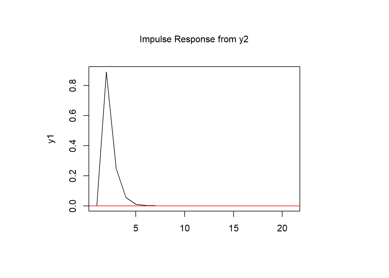
参照引用資料
- 村尾博(2019),『Rで学ぶVAR実証分析』,オーム社,pp.288-293
最終更新
Sys.time()[1] "2024-04-16 10:13:16 JST"R、Quarto、Package
R.Version()$version.string[1] "R version 4.3.3 (2024-02-29 ucrt)"quarto::quarto_version()[1] '1.4.553'packageVersion(pkg = "tidyverse")[1] '2.0.0'