library(ggplot2)
library(dplyr)
seed <- 20230323Rで回帰分析:一般化線形モデル(誤差構造:ガンマ分布)
Rでデータサイエンス
一般化線形モデル(誤差構造:ガンマ分布)
リンク関数:log
# サンプルデータの作成
set.seed(seed)
n <- 100
# 説明変数
x1 <- runif(n = n, min = -1, max = 1)
x2 <- runif(n = n, min = -1, max = 1)
# 偏回帰係数
b0 <- 5
b1 <- 3
b2 <- -4
# 目的変数
y0 <- exp((cbind(x1, x2) %*% c(b1, b2)) + b0)
shape <- 5
y <- rgamma(n = n, shape = shape, rate = shape/y0)
glimpse(data.frame(x1, x2, y0, y))
Rows: 100
Columns: 4
$ x1 <dbl> 0.09833080, 0.40809112, -0.28402327, -0.02762073, -0.32627147, 0.50…
$ x2 <dbl> -0.156941584, -0.616776818, 0.655992050, 0.631932357, 0.181449611, …
$ y0 <dbl> 373.4405194, 5951.3932412, 4.5903763, 10.9070392, 26.9878599, 673.4…
$ y <dbl> 659.0549817, 7727.3539720, 2.4001331, 3.1500989, 25.6641597, 1059.3…result <- glm(formula = y ~ x1 + x2, family = Gamma(link = "log"))
result %>%
summary()
Call:
glm(formula = y ~ x1 + x2, family = Gamma(link = "log"))

Coefficients:
            Estimate Std. Error t value            Pr(>|t|)
(Intercept)  4.94651    0.04740  104.35 <0.0000000000000002 ***
x1           3.00906    0.08925   33.72 <0.0000000000000002 ***
x2          -3.99224    0.08342  -47.86 <0.0000000000000002 ***
---
Signif. codes:  0 '***' 0.001 '**' 0.01 '*' 0.05 '.' 0.1 ' ' 1

(Dispersion parameter for Gamma family taken to be 0.2219225)

    Null deviance: 608.567  on 99  degrees of freedom
Residual deviance:  24.988  on 97  degrees of freedom
AIC: 1082

Number of Fisher Scoring iterations: 5confint(object = result, level = 0.95) 2.5 % 97.5 %
(Intercept) 4.854998 5.040939
x1 2.828907 3.190383
x2 -4.157127 -3.827821リンク関数:inverse
# サンプルデータの作成
set.seed(seed)
# 説明変数
n <- 100
x_min <- 1
x_max <- 5
x <- runif(n = n, min = x_min, max = x_max)
# 目的変数
b0 <- 8
b1 <- 5
y0 <- b1 * x + b0
# shape と rate 毎の形状の確認
# https://qiita.com/hoxo_b/items/a6522a6e6561f8ca7b96
parm <- expand.grid(shape = c(1, 2), rate = c(1, 2))
ggplot(data = data.frame(x = c(x_min, x_max)), mapping = aes(x = x)) + mapply(FUN = function(shape, rate, linetype) {
stat_function(fun = dgamma, args = list(shape = shape, rate = rate), mapping = aes(linetype = linetype))
}, parm$shape, parm$rate, sprintf("shape=%.0f rate=%.1f", parm$shape, parm$rate)) + labs(linetype = "parameter") + theme_minimal()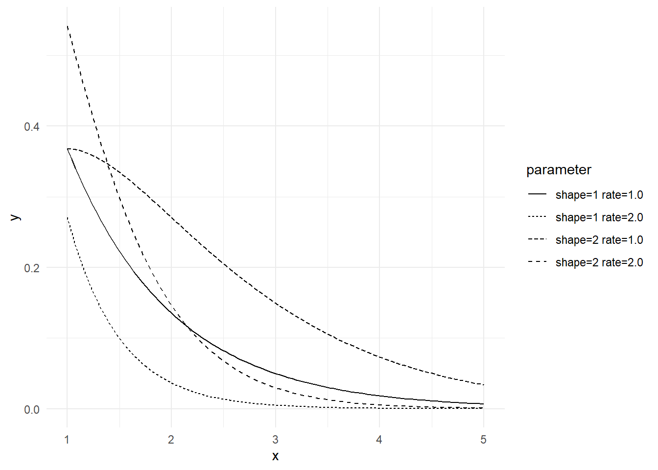
shape <- 2
# y <- rgamma(n = n,shape = shape,scale = 1/y0/shape)
y <- rgamma(n = n, shape = shape, rate = y0 * shape)
result <- glm(formula = y ~ x, family = Gamma(link = "inverse"))
summary(result)
Call:
glm(formula = y ~ x, family = Gamma(link = "inverse"))

Coefficients:
            Estimate Std. Error t value Pr(>|t|)
(Intercept)    8.728      4.313   2.023  0.04575 *
x              5.079      1.660   3.060  0.00286 **
---
Signif. codes:  0 '***' 0.001 '**' 0.01 '*' 0.05 '.' 0.1 ' ' 1

(Dispersion parameter for Gamma family taken to be 0.5622483)

    Null deviance: 69.463  on 99  degrees of freedom
Residual deviance: 63.998  on 98  degrees of freedom
AIC: -433.15

Number of Fisher Scoring iterations: 6confint(object = result, level = 0.95) 2.5 % 97.5 %
(Intercept) 0.6506416 17.544930
x 1.8635415 8.370862# 回帰曲線
b0_bar <- result$coefficients[1]
b1_bar <- result$coefficients[2]
ggplot(data = data.frame(x, y), mapping = aes(x = x, y = y)) + geom_point() + geom_smooth(method = "glm", method.args = list(family = Gamma(link = "inverse")), color = "blue", linewidth = 1, se = F) + stat_function(fun = function(x) 1/(b1_bar * x + b0_bar), color = "red", linewidth = 1, linetype = "dashed") + theme_minimal()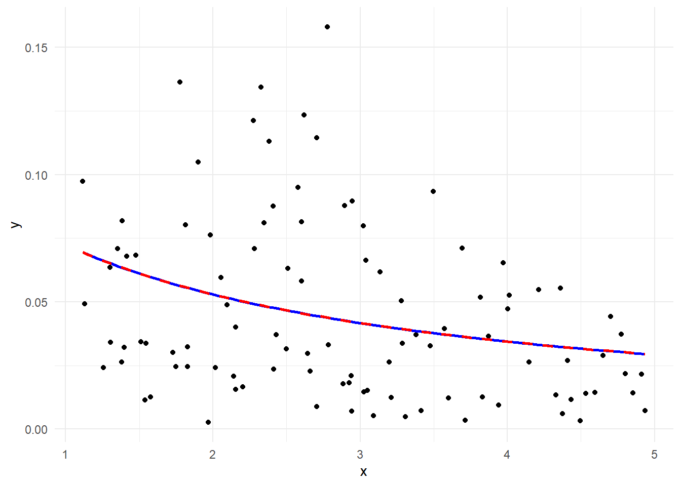
参考引用資料
最終更新
Sys.time()[1] "2024-03-30 05:49:30 JST"R、Quarto、Package
R.Version()$version.string[1] "R version 4.3.3 (2024-02-29 ucrt)"quarto::quarto_version()[1] '1.4.542'packageVersion(pkg = "tidyverse")[1] '2.0.0'