library(ggplot2)
library(dplyr)
seed <- 20230325Rで回帰分析:一般化線形モデル(誤差構造:ポアソン分布)
Rでデータサイエンス
一般化線形モデル(誤差構造:ポアソン分布)
リンク関数:identity
# サンプルデータの作成
set.seed(seed)
b <- c(5, 3)  # 偏回帰係数
n <- 100  # サンプルサイズ
x1 <- runif(n = n)  # 説明変数
x2 <- runif(n = n)  # 説明変数
z <- (cbind(x1, x2) %*% b)
z %>%
    range()
[1] 1.094293 7.659596# 目的変数の作成とヒストグラム
y <- rpois(n = n, lambda = z)
ggplot(mapping = aes(x = y)) + geom_histogram(binwidth = 1, fill = "skyblue", col = "black") + theme_minimal() + scale_x_continuous(breaks = scales::pretty_breaks(10))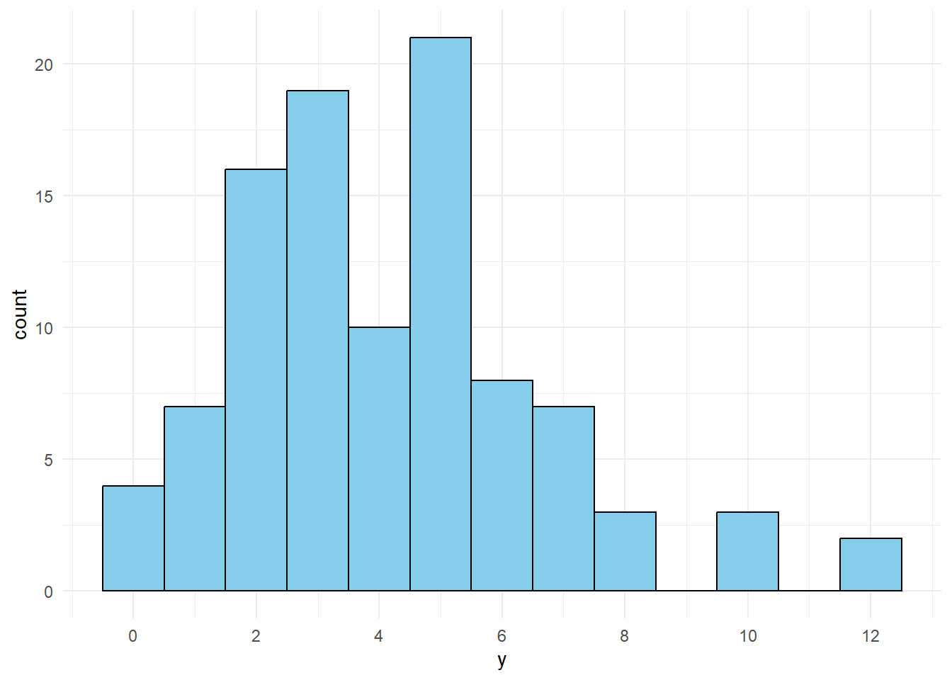
data.frame(x1, x2, z, y) %>%
    glimpse()
Rows: 100
Columns: 4
$ x1 <dbl> 0.60698381, 0.51033524, 0.90677612, 0.96388536, 0.92631483, 0.43880…
$ x2 <dbl> 0.58054902, 0.97128861, 0.40884385, 0.44383869, 0.02527208, 0.47889…
$ z <dbl> 4.776566, 5.465542, 5.760412, 6.150943, 4.707390, 3.630736, 3.72243…
$ y <int> 2, 6, 6, 7, 3, 2, 1, 5, 2, 6, 5, 3, 3, 4, 7, 2, 1, 5, 5, 3, 2, 7, 3…result <- glm(formula = y ~ x1 + x2 - 1, family = poisson(link = "identity"))
result %>%
summary()
Call:
glm(formula = y ~ x1 + x2 - 1, family = poisson(link = "identity"))

Coefficients:
   Estimate Std. Error z value             Pr(>|z|)
x1   4.5118     0.4747   9.505 < 0.0000000000000002 ***
x2   3.1827     0.4738   6.717      0.0000000000185 ***
---
Signif. codes:  0 '***' 0.001 '**' 0.01 '*' 0.05 '.' 0.1 ' ' 1

(Dispersion parameter for poisson family taken to be 1)

    Null deviance:    Inf  on 100  degrees of freedom
Residual deviance: 115.13  on  98  degrees of freedom
AIC: 426.41

Number of Fisher Scoring iterations: 6confint(result) 2.5 % 97.5 %
x1 3.593609 5.474191
x2 2.287620 4.166084リンク関数:log
# サンプルデータの作成
set.seed(seed)
n <- 100  # サンプルサイズ
b0 <- 5
b1 <- -2
x <- runif(n = n)
z <- exp(x * b1 + b0)
z %>%
    range()
[1] 20.60722 147.94512y <- rpois(n = n, lambda = z)
ggplot(mapping = aes(x = y)) + geom_histogram(binwidth = 10, fill = "skyblue", col = "black") + theme_minimal() + scale_x_continuous(breaks = scales::pretty_breaks(20))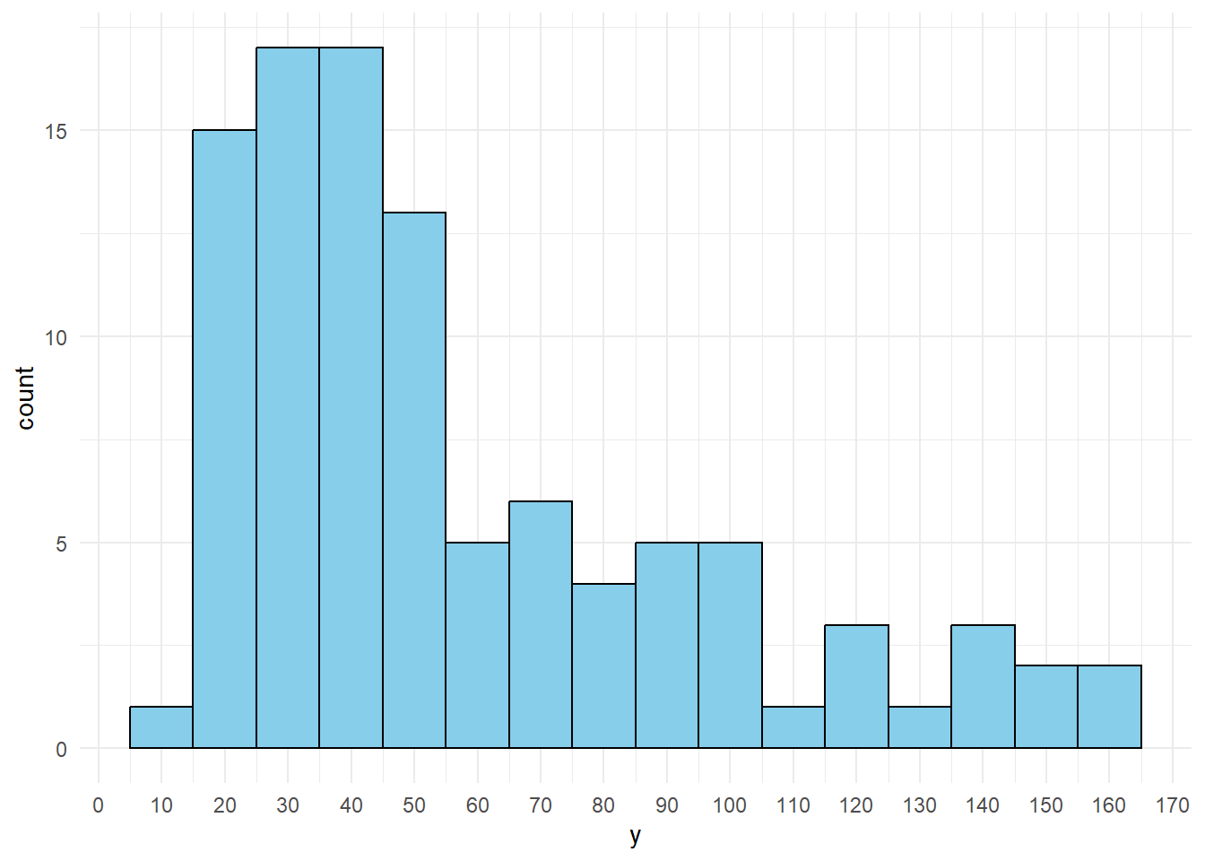
data.frame(x, y) %>%
    glimpse()
Rows: 100
Columns: 2
$ x <dbl> 0.60698381, 0.51033524, 0.90677612, 0.96388536, 0.92631483, 0.438807…
$ y <int> 45, 51, 23, 22, 19, 58, 36, 50, 100, 21, 38, 37, 48, 25, 70, 132, 52…result <- glm(formula = y ~ x, family = poisson(link = "log"))
result %>%
summary()
Call:
glm(formula = y ~ x, family = poisson(link = "log"))

Coefficients:
            Estimate Std. Error z value            Pr(>|z|)
(Intercept)  4.99920    0.02156  231.90 <0.0000000000000002 ***
x           -1.98444    0.04483  -44.26 <0.0000000000000002 ***
---
Signif. codes:  0 '***' 0.001 '**' 0.01 '*' 0.05 '.' 0.1 ' ' 1

(Dispersion parameter for poisson family taken to be 1)

    Null deviance: 2123.68  on 99  degrees of freedom
Residual deviance:  112.78  on 98  degrees of freedom
AIC: 689.37

Number of Fisher Scoring iterations: 4confint(result) 2.5 % 97.5 %
(Intercept) 4.956725 5.041232
x -2.072443 -1.896687b0_bar <- result$coefficients[1]
b1_bar <- result$coefficients[2]
ggplot(data = data.frame(x, y), mapping = aes(x = x, y = y)) + geom_point() + geom_smooth(method = "glm", method.args = list(family = poisson(link = "log")), se = F, color = "blue", linewidth = 1) + stat_function(fun = function(x) exp(x * b1 + b0), color = "red", linewidth = 1, linetype = "dashed") + theme_minimal()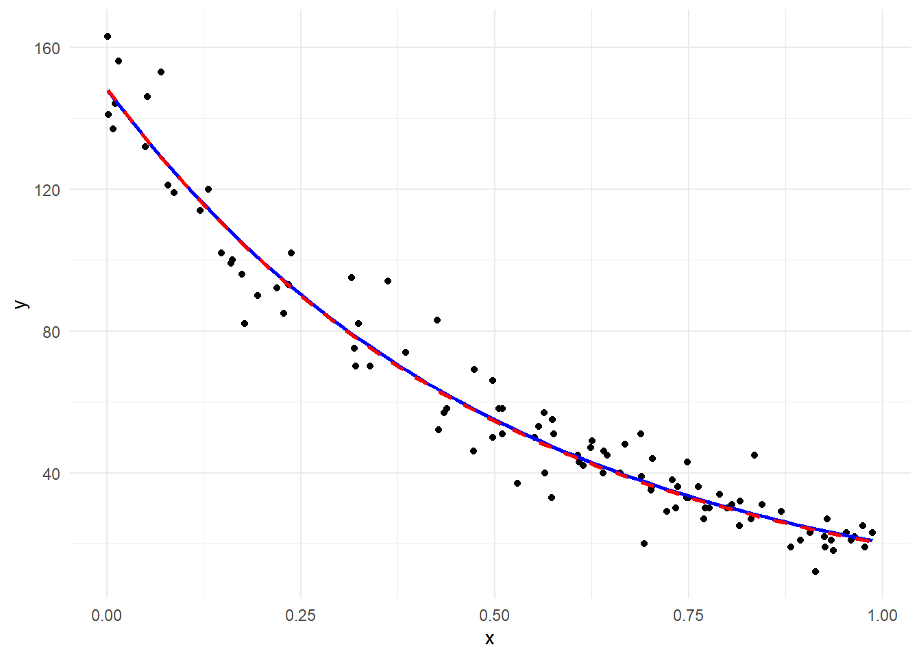
参考引用資料
最終更新
Sys.time()[1] "2024-04-01 06:34:17 JST"R、Quarto、Package
R.Version()$version.string[1] "R version 4.3.3 (2024-02-29 ucrt)"quarto::quarto_version()[1] '1.4.542'packageVersion(pkg = "tidyverse")[1] '2.0.0'