# サンプルデータの作成
library(sandwich)
library(dplyr)
seed <- 20230414
set.seed(seed)
n <- 50
x <- runif(n = n)
x <- seq(from = 0.1, to = 1, length.out = n)
num_sd <- runif(n = n, min = 0.1, max = 1.5)
e <- num_sd %>%
    rnorm(n = n, sd = .)
b1 <- 2
b0 <- 4
y <- b0 * x + b1 + eRで回帰分析:ロバスト標準誤差
Rでデータサイエンス
ロバスト標準誤差
ロバスト(頑健)なt統計量を求めるには推定された回帰係数の分散不均一の時の一致性のある標準誤差が必要である。
Whiteの修正
以下の関係を考えたとき
\[ \begin{equation} y_i=b_1+b_0 x_i+e_i \tag{1} \end{equation} \]
OLS推定量は
\[ \begin{equation} \hat{b_0}=b_0+\dfrac{\displaystyle\sum_{i=1}^n\left(x_i-\bar{\textbf{x}}\right)e_i}{\displaystyle\sum_{i=1}^n\left(x_i-\bar{\textbf{x}}\right)^2} \tag{2} \end{equation} \] となり\(\,\hat{b_0}\,\)は以下の通りに不編性を満たす。
\[ \begin{equation} \textrm{E}\left[\hat{b_0}\right]=b_0+\dfrac{\displaystyle\sum_{i=1}^n\left(x_i-\bar{\textbf{x}}\right)\textrm{E}\left[e_i\right]}{\displaystyle\sum_{i=1}^n\left(x_i-\bar{\textbf{x}}\right)^2}=b_0 \tag{3} \end{equation} \] ここで\(\,\textrm{E}\left[e_i\right]=0\,\)である。
誤差項の分散が均一であれば
\[ \begin{equation} \textrm{var}(\hat{b_0})=\dfrac{\sigma^2}{\displaystyle\sum_{i=1}^n\left(x_i-\bar{\textbf{x}}\right)^2} \tag{4} \end{equation} \]
であるが、不均一の場合は
\[ \begin{equation} \textrm{var}(e_i)=\sigma_i^2=\sigma^2z_i^2 \tag{5} \end{equation} \] であることから、(4)式に代入すると
\[ \begin{equation} \textrm{var}(\hat{b_0}) =\dfrac{\displaystyle\sum_{i=1}^n\left(x_i-\bar{\textbf{x}}\right)^2\sigma_i^2}{\left(\displaystyle\sum_{i=1}^n\left(x_i-\bar{\textbf{x}}\right)^2\right)^2} =\dfrac{\sigma^2\displaystyle\sum_{i=1}^n\left(x_i-\bar{\textbf{x}}\right)^2z_i^2}{\left(\displaystyle\sum_{i=1}^n\left(x_i-\bar{\textbf{x}}\right)^2\right)^2} \tag{6} \end{equation} \] 但し\(\,\sigma_i^2\,\)は未知であるが、観察可能な\(\,e_i\,\)を用いるのが以下のWhiteの修正。
\[ \begin{equation} \textrm{var}(\hat{b_0}) =\dfrac{\displaystyle\sum_{i=1}^n\left(x_i-\bar{\textbf{x}}\right)^2\hat{e}_i^2}{\left(\displaystyle\sum_{i=1}^n\left(x_i-\bar{\textbf{x}}\right)^2\right)^2} \tag{7} \end{equation} \] ここで\(\,\hat{e}_i=y_i-\hat{b_1}-\hat{b_0}x_i\,\)であり、サンプルサイズが大きくなるに従い分母は\(\,\infty\,\)に近づき\(\,\textrm{V}(\hat{b_0})\,\)はゼロに収束し、さらにOLS推定量は一致性も満たす。
この平方根は
- 分散不均一の時の一致性のある標準誤差
- 不均一分散一致標準誤差
- 不均一分散頑強標準誤差
- ロバスト標準誤差
- ホワイト標準誤差
- Heteroskedasticity-consistent standard errors
等と呼ばれ、 \[ \begin{equation} t=\dfrac{\hat{b}-b}{\sqrt{\textrm{var}(\hat{b}_0)}} \tag{8} \end{equation} \] を利用してt検定を行う。
以上は
- https://ir.lib.hiroshima-u.ac.jp/files/public/2/26959/20141016155608105544/YuseiKenkyushoGeppo_12-7_156.pdf
- https://www.fbc.keio.ac.jp/~tyabu/econometrics/econome1_9.pdf
から多くを引用している。
サンプルデータの作成
分散の不均一を考慮しない場合の回帰式の区間推定
# 分散の不均一を考慮しない場合の回帰式の区間推定
library(ggplot2)
(g <- ggplot(data = data.frame(x, y), mapping = aes(x = x, y = y)) + geom_point() + geom_smooth(method = "lm") + theme_minimal())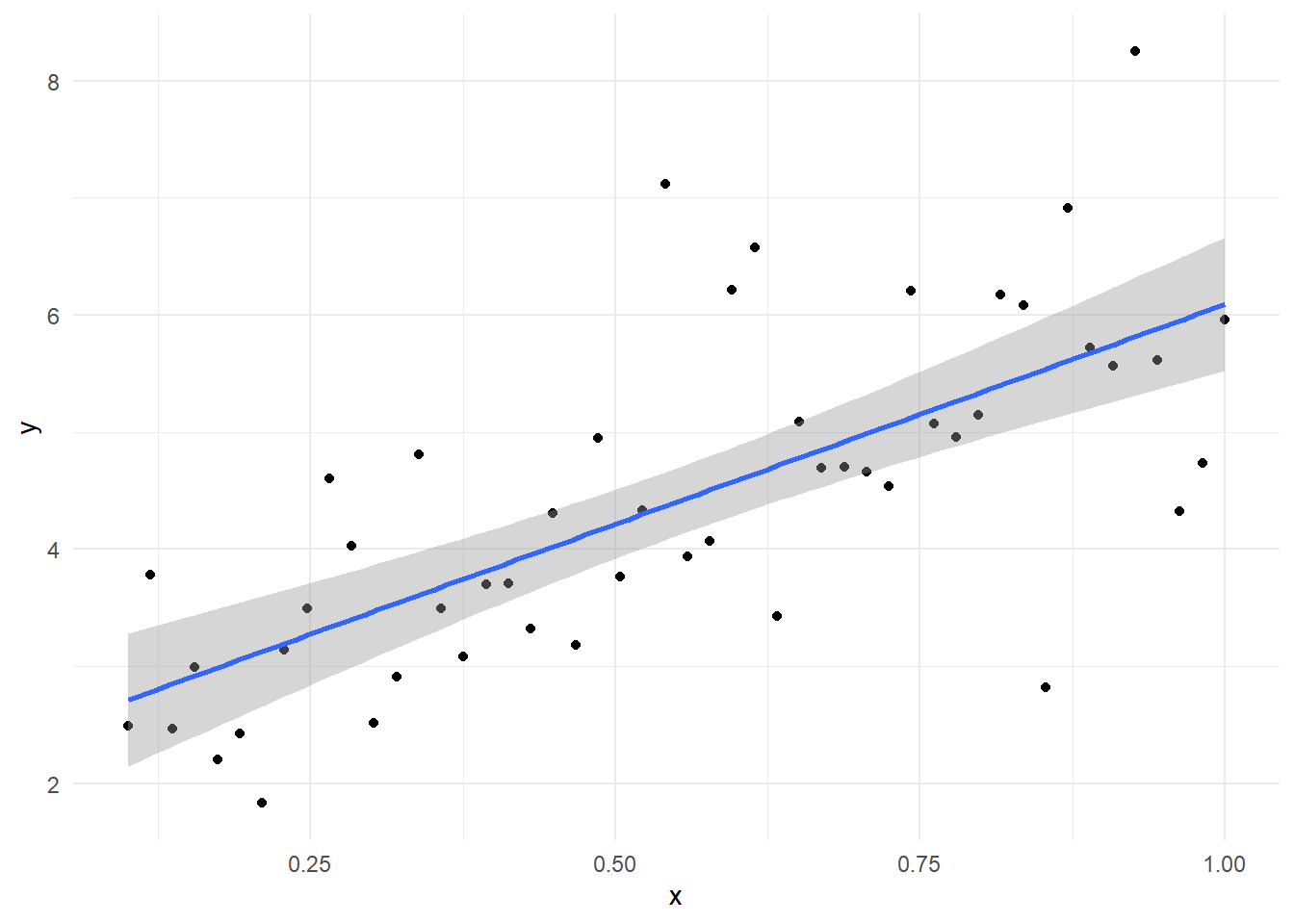
誤差項の分散不均一を考慮せずに母回帰式の区間推定を求める関数
fun_ci_of_population_regression <- function(x, y, n) {
    # 誤差項の分散不均一を考慮せずに母回帰式の区間推定を求める関数
    # 有意水準
    significant_level <- 0.05
    # 自由度 n-2、有意水準 0.05 の t 値
    t_value <- qt(1 - significant_level/2, n - 2)
    # 説明変数 x の偏差平方和
    Sxx <- sum((x - mean(x))^2)
    # 説明変数 x と目的変数 y の積和
    Sxy <- sum((x - mean(x)) * (y - mean(y)))
    # 回帰直線の傾きの推定量
    b0_hat <- Sxy/Sxx
    # 回帰直線の切片の推定量
    b1_hat <- mean(y) - mean(x) * b0_hat
    # 推定された y
    estimated_y <- b0_hat * x + b1_hat
    # 残差
    residuals <- y - estimated_y
    # 残差標準偏差
    sigma <- sqrt(sum((residuals - mean(residuals))^2)/(n - 2))
    # 信頼区間
    ci <- t_value * sqrt(1/n + ((x - mean(x))^2)/Sxx) * sigma
    # 下限
    lower_limit <- estimated_y - ci
    # 上限
    upper_limit <- estimated_y + ci
    return(list(lower_limit = lower_limit, upper_limit = upper_limit, b0_hat = b0_hat, b1_hat = b1_hat))
}
(limit <- fun_ci_of_population_regression(x = x, y = y, n = n))$lower_limit
[1] 2.143079 2.229214 2.315150 2.400867 2.486344 2.571554 2.656472 2.741066
[9] 2.825302 2.909140 2.992538 3.075448 3.157816 3.239583 3.320684 3.401050
[17] 3.480605 3.559271 3.636965 3.713605 3.789112 3.863409 3.936432 4.008125
[25] 4.078452 4.147393 4.214947 4.281135 4.345994 4.409578 4.471953 4.533194
[33] 4.593382 4.652597 4.710924 4.768439 4.825219 4.881334 4.936848 4.991819
[41] 5.046303 5.100346 5.153991 5.207279 5.260243 5.312913 5.365318 5.417483
[49] 5.469428 5.521174
$upper_limit
[1] 3.284117 3.335863 3.387808 3.439973 3.492378 3.545049 3.598012 3.651300
[9] 3.704946 3.758989 3.813472 3.868444 3.923957 3.980072 4.036852 4.094368
[17] 4.152694 4.211910 4.272097 4.333338 4.395713 4.459297 4.524156 4.590344
[25] 4.657898 4.726839 4.797166 4.868860 4.941882 5.016179 5.091686 5.168326
[33] 5.246020 5.324686 5.404241 5.484607 5.565708 5.647475 5.729843 5.812753
[41] 5.896151 5.979989 6.064225 6.148819 6.233737 6.318948 6.404424 6.490141
[49] 6.576077 6.662212
$b0_hat
[1] 3.753439
$b1_hat
[1] 2.338254(g <- g + geom_line(data = data.frame(x = x, y = limit$upper_limit), mapping = aes(x = x, y = limit$upper_limit), linewidth = 1, col = "red", linetype = "dashed") + geom_line(data = data.frame(x = x, y = limit$lower_limit), mapping = aes(x = x, y = limit$lower_limit), linewidth = 1, col = "red", linetype = "dashed"))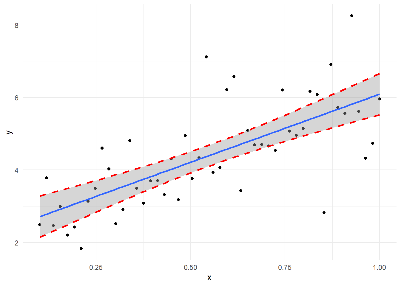
result <- lm(y ~ x)
result %>%
    summary()
Call:
lm(formula = y ~ x)

Residuals:
    Min      1Q  Median      3Q     Max
-2.7193 -0.5136 -0.1796  0.5342  2.7547

Coefficients:
            Estimate Std. Error t value      Pr(>|t|)
(Intercept)   2.3383     0.3317   7.049 0.00000000618 ***
x             3.7534     0.5433   6.908 0.00000001016 ***
---
Signif. codes:  0 '***' 0.001 '**' 0.01 '*' 0.05 '.' 0.1 ' ' 1

Residual standard error: 1.018 on 48 degrees of freedom
Multiple R-squared:  0.4986,    Adjusted R-squared:  0.4881
F-statistic: 47.73 on 1 and 48 DF,  p-value: 0.00000001016
誤差項の分散不均一を考慮した回帰モデル
# 誤差項の分散不均一を考慮した回帰モデル
library(estimatr)
lm_robust(y ~ x, se_type = "HC0")
# Estimate は変わらない。
# Std.Error は異なる。
# HC0:White(1980)
Estimate Std. Error t value Pr(>|t|) CI Lower CI Upper
(Intercept) 2.338254 0.2744897 8.518548 0.00000000003665655 1.786355 2.890153
x 3.753439 0.5355620 7.008412 0.00000000713800728 2.676620 4.830259
DF
(Intercept) 48
x 48# 赤色ダッシュが誤差項の分散不均一を考慮しない場合の区間推定
# 青色塗りつぶしは誤差項の分散不均一を考慮した場合の区間推定
ggplot(data = data.frame(x, y), mapping = aes(x = x, y = y)) + geom_point() + theme_minimal() + geom_smooth(method = "lm_robust", fill = "blue", alpha = 0.15, method.args = list(se_type = "HC0")) + geom_line(data = data.frame(x = x, y = limit$upper_limit), mapping = aes(x = x, y = limit$upper_limit), linewidth = 1, col = "red", linetype = "dashed") + geom_line(data = data.frame(x = x, y = limit$lower_limit), mapping = aes(x = x, y = limit$lower_limit), linewidth = 1, col = "red", linetype = "dashed")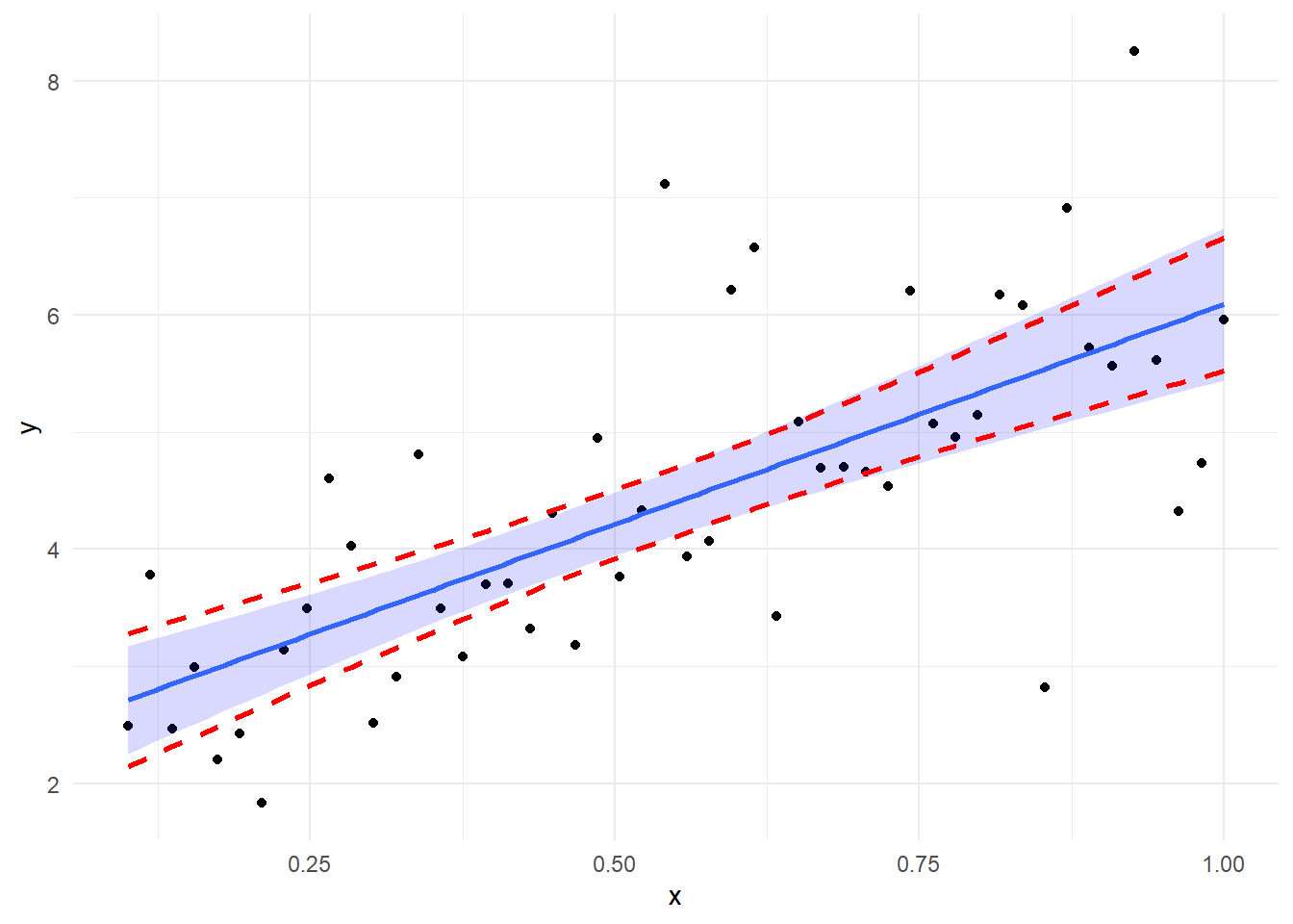
# sandwich関数を利用して同じ結果を得る
(result_vcov <- sandwich::vcovHC(result, type = "HC0"))
(Intercept) x
(Intercept) 0.07534461 -0.1292733
x -0.12927331 0.2868267lmtest::coeftest(x = result, vcov. = result_vcov)
t test of coefficients:

            Estimate Std. Error t value         Pr(>|t|)
(Intercept)  2.33825    0.27449  8.5185 0.00000000003666 ***
x            3.75344    0.53556  7.0084 0.00000000713801 ***
---
Signif. codes:  0 '***' 0.001 '**' 0.01 '*' 0.05 '.' 0.1 ' ' 1
参考引用資料
- https://www.ier.hit-u.ac.jp/~kitamura/lecture/Hit/08Statsys4.pdf#page=4
- https://www.fbc.keio.ac.jp/~tyabu/econometrics/econome1_9.pdf
- https://declaredesign.org/r/estimatr/articles/mathematical-notes.html
- https://cran.r-project.org/web/packages/sandwich/vignettes/sandwich.pdf
- https://www.reed.edu/economics/parker/s12/312/notes/Notes8.pdf
- https://hermes-ir.lib.hit-u.ac.jp/hermes/ir/re/15457/keizai0010100010.pdf
- https://ir.lib.hiroshima-u.ac.jp/files/public/2/26959/20141016155608105544/YuseiKenkyushoGeppo_12-7_156.pdf
- https://nigimitama.hatenablog.jp/entry/2019/01/26/010612
最終更新
Sys.time()[1] "2024-03-24 06:19:42 JST"R、Quarto、Package
R.Version()$version.string[1] "R version 4.3.3 (2024-02-29 ucrt)"quarto::quarto_version()[1] '1.4.542'packageVersion(pkg = "tidyverse")[1] '2.0.0'