トービット・モデル
\[
\begin{eqnarray}
\textrm{y}_i^{\ast}&=&\mathrm{\beta\,x}_i+\textrm{u}_i\\
\textrm{y}_i &=&\left\{
\begin{array}{ll}
0 & (\textrm{y}^{\ast}_i \leq 0)\\
\textrm{y}^{\ast}_i & (\textrm{y}^{\ast}_i >0)
\end{array}
\right.
\end{eqnarray}
\] 『通常の最小二乗法による推定量はバイアスがあることが知られており,最小二乗法は\(\,\mathrm{\beta}\,\)の推定に使うことはできず,最尤法に基づく推定量が推定に用いられる。』 - 出所: https://dl.ndl.go.jp/view/prepareDownload?itemId=info%3Andljp%2Fpid%2F11172411&contentNo=1
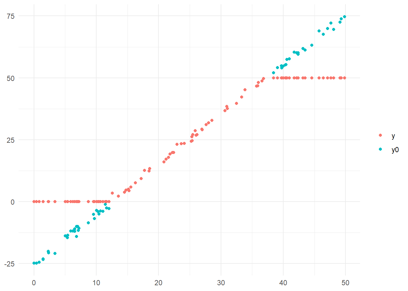
サンプルデータの作成
# サンプルデータの作成
library(VGAM)
library(dplyr)
library(ggplot2)
set.seed(20230426)
n <- 100
x <- runif(n = n, min = 0, max = 50)
b0 <- -25
b1 <- 2
y0 <- b0 + b1 * x + rnorm(n = n)
y <- y0 %>%
    {
        ifelse(. > 50, 50, ifelse(. < 0, 0, .))
    }
tidydf <- data.frame(x, y0, y) %>%
    {
        tidyr::gather(data = ., key = "key", value = "value", colnames(.)[-1])
    }
(g <- ggplot(data = tidydf, mapping = aes(x = x, y = value, col = key)) + geom_point() + theme_minimal() + theme(legend.title = element_blank(), axis.title = element_blank()))
トービット・モデル
# トービット・モデル
model_tobit_censored <- vglm(y ~ x, family = tobit(Lower = 0, Upper = 50, type.fitted = "censored"), trace = T)
model_tobit_censored %>%
    summary()
VGLM    linear loop  1 :  loglikelihood = -59.795084
VGLM    linear loop  2 :  loglikelihood = -58.963179
VGLM    linear loop  3 :  loglikelihood = -58.94609
VGLM    linear loop  4 :  loglikelihood = -58.946045
VGLM    linear loop  5 :  loglikelihood = -58.946044

Call:
vglm(formula = y ~ x, family = tobit(Lower = 0, Upper = 50, type.fitted = "censored"),
    trace = T)

Coefficients:
               Estimate Std. Error z value            Pr(>|z|)
(Intercept):1 -25.09608    0.49066 -51.148 <0.0000000000000002 ***
(Intercept):2  -0.09271    0.10614  -0.874               0.382
x               2.02091    0.01936 104.403 <0.0000000000000002 ***
---
Signif. codes:  0 '***' 0.001 '**' 0.01 '*' 0.05 '.' 0.1 ' ' 1

Names of linear predictors: mu, loglink(sd)

Log-likelihood: -58.946 on 197 degrees of freedom

Number of Fisher scoring iterations: 5

Warning: Hauck-Donner effect detected in the following estimate(s):
'(Intercept):1'
打ち切りなしの最尤推定
# 打ち切りなしの最尤推定
model_tobit_uncensored <- vglm(y ~ x, family = tobit(Lower = -Inf, Upper = Inf, type.fitted = "uncensored"), trace = T)
model_tobit_uncensored %>%
    summary()
VGLM    linear loop  1 :  loglikelihood = -298.80209
VGLM    linear loop  2 :  loglikelihood = -297.19837
VGLM    linear loop  3 :  loglikelihood = -297.17209
VGLM    linear loop  4 :  loglikelihood = -297.17209
VGLM    linear loop  5 :  loglikelihood = -297.17209

Call:
vglm(formula = y ~ x, family = tobit(Lower = -Inf, Upper = Inf,
    type.fitted = "uncensored"), trace = T)

Coefficients:
              Estimate Std. Error z value            Pr(>|z|)
(Intercept):1 -9.35191    0.88801  -10.53 <0.0000000000000002 ***
(Intercept):2  1.55278    0.07071   21.96 <0.0000000000000002 ***
x              1.37773    0.03219   42.80 <0.0000000000000002 ***
---
Signif. codes:  0 '***' 0.001 '**' 0.01 '*' 0.05 '.' 0.1 ' ' 1

Names of linear predictors: mu, loglink(sd)

Log-likelihood: -297.1721 on 197 degrees of freedom

Number of Fisher scoring iterations: 5

No Hauck-Donner effect found in any of the estimates
最小二乗法による線形回帰
# 最小二乗法による線形回帰
model_ols <- lm(y ~ x)
model_ols %>%
    summary()
Call:
lm(formula = y ~ x)

Residuals:
    Min      1Q  Median      3Q     Max
-9.2938 -3.8934  0.2396  3.6403  9.2993

Coefficients:
            Estimate Std. Error t value            Pr(>|t|)
(Intercept) -9.35191    0.89703  -10.43 <0.0000000000000002 ***
x            1.37773    0.03252   42.37 <0.0000000000000002 ***
---
Signif. codes:  0 '***' 0.001 '**' 0.01 '*' 0.05 '.' 0.1 ' ' 1

Residual standard error: 4.773 on 98 degrees of freedom
Multiple R-squared:  0.9482,    Adjusted R-squared:  0.9477
F-statistic:  1795 on 1 and 98 DF,  p-value: < 0.00000000000000022
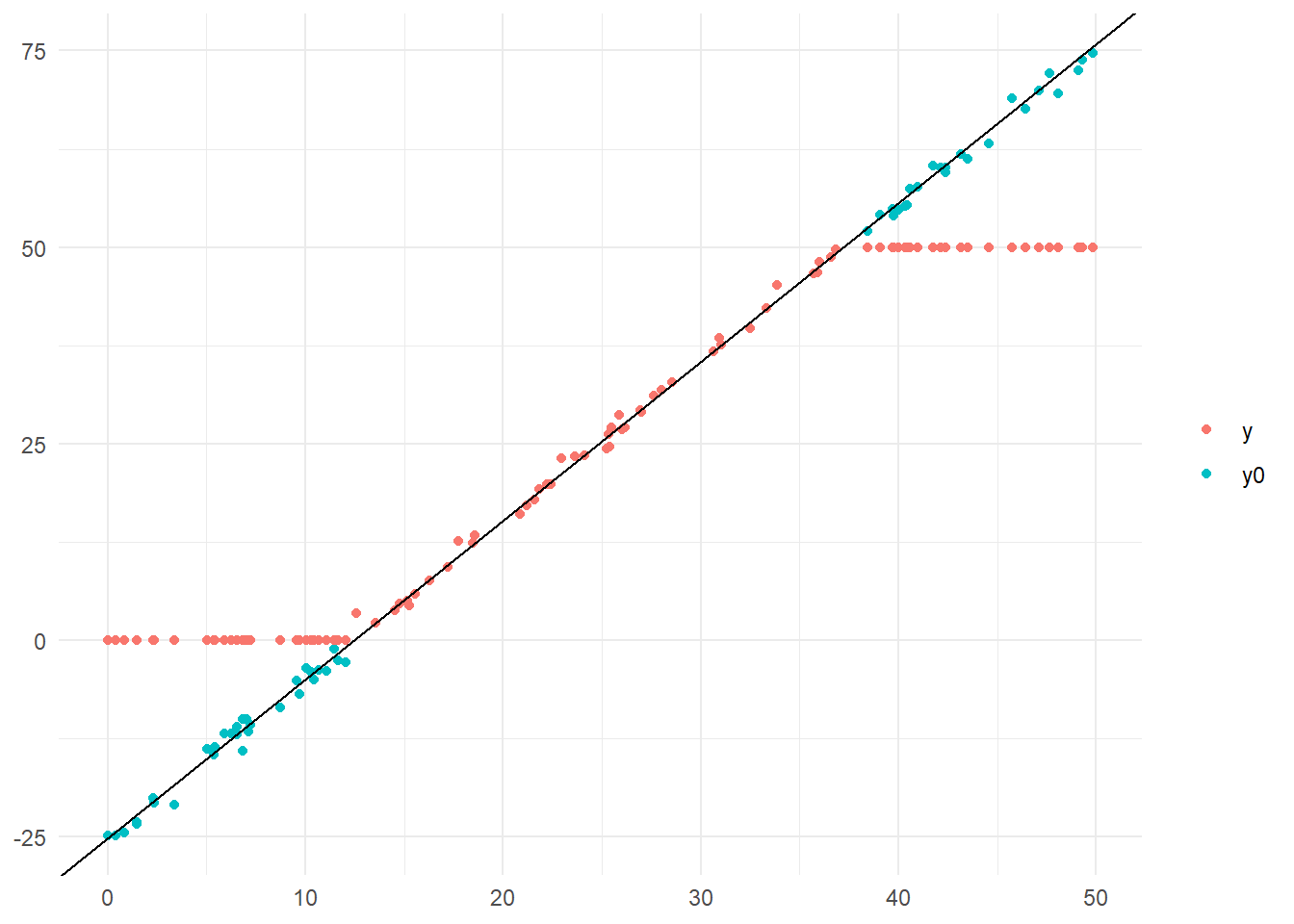
結果の散布図と回帰直線
トービット・モデル
# トービット・モデル
g + geom_abline(intercept = coef(model_tobit_censored)[c(1)], slope = coef(model_tobit_censored)[c(3)])
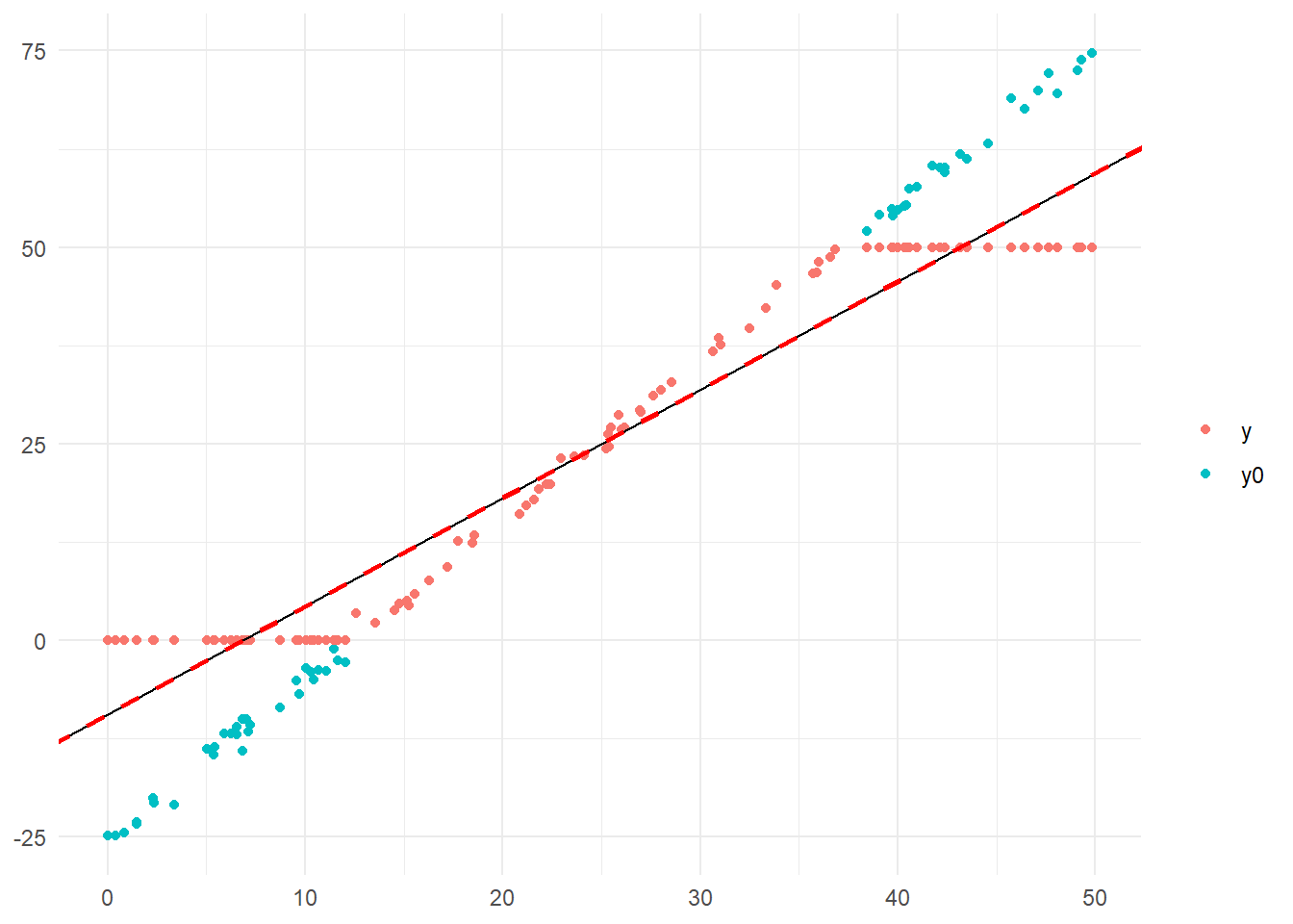
最小二乗法による線形回帰と打ち切りなしの最尤推定
# 最小二乗法による線形回帰と打ち切りなしの最尤推定
g + geom_abline(intercept = coef(model_tobit_uncensored)[c(1)], slope = coef(model_tobit_uncensored)[c(3)]) + geom_abline(intercept = coef(model_ols)[c(1)], slope = coef(model_ols)[c(2)], linetype = "dashed", col = "red", linewidth = 1)
最終更新
[1] "2024-03-25 08:31:00 JST"
R、Quarto、Package
R.Version()$version.string
[1] "R version 4.3.3 (2024-02-29 ucrt)"
packageVersion(pkg = "tidyverse")
著者
Figure 1:
Figure 2:
Figure 3: