Rで季節調整

Rでデータサイエンス

library(seasonal)
packageVersion("seasonal")

[1] '1.9.0'

サンプルデータ

2018年1月から2023年12月までの業種別鉱工業生産指数(ウエイト:10000)をサンプルデータとします。
2020年基準鉱工業指数統計表一覧
鉱工業指数のしくみと見方
鉱工業指数:IIP(Indices of Industrial Production)
以下有意水準は全て5%とする。

rbind(head(df_iip), tail(df_iip))

         date IIP_NSA IIP_SA
1  2018-01-01   105.6  112.3
2  2018-02-01   111.0  114.6
3  2018-03-01   128.1  116.3
4  2018-04-01   111.8  114.5
5  2018-05-01   109.9  115.1
6  2018-06-01   115.5  114.3
67 2023-07-01   105.1  103.5
68 2023-08-01    96.1  103.1
69 2023-09-01   107.0  103.2
70 2023-10-01   106.3  104.4
71 2023-11-01   106.9  103.8
72 2023-12-01   106.4  105.0

df_iip %>%
    gather(key = "IIP", value = "value", colnames(.)[-1]) %>%
    ggplot(mapping = aes(x = date, y = value, col = IIP)) + geom_point() + geom_line()

# ts class に変換
(iip_nsa <- df_iip$IIP_NSA %>%
    ts(start = df_iip$date %>%
        head(1) %>%
        {
            c(year(.), month(.))
        }, end = df_iip$date %>%
        tail(1) %>%
        {
            c(year(.), month(.))
        }, frequency = 12))

       Jan   Feb   Mar   Apr   May   Jun   Jul   Aug   Sep   Oct   Nov   Dec
2018 105.6 111.0 128.1 111.8 109.9 115.5 117.0 108.0 113.8 120.2 119.0 115.7
2019 106.0 110.4 122.9 111.4 107.9 111.9 118.2 102.6 115.9 110.8 109.7 111.4
2020 102.7 103.7 116.5  94.8  80.0  91.6  99.1  87.9 104.6 106.2 104.8 107.9
2021  97.4 101.4 120.1 108.4  95.4 111.6 109.9  95.4 103.1 102.2 110.1 110.0
2022  96.7 101.4 118.2 103.3  92.8 108.3 107.9 100.8 112.1 105.4 108.6 107.6
2023  93.8 100.9 117.3 102.5  96.6 108.2 105.1  96.1 107.0 106.3 106.9 106.4

季節調整:SEATSによる

sa <- seas(x = iip_nsa)
sa %>%
    plot()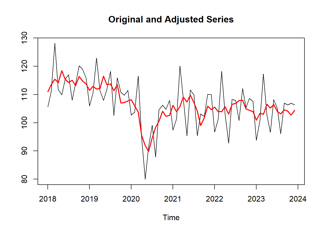

Tip

デフォルトの季節調整はSEATSが選択される。

summary(sa)


Call:
seas(x = iip_nsa)

Coefficients:
                  Estimate Std. Error z value             Pr(>|z|)    
Leap Year           1.3553     2.2302   0.608               0.5434    
Weekday             0.4795     0.0707   6.783      0.0000000000118 ***
AR-Nonseasonal-01   0.7637     0.1694   4.507      0.0000065622008 ***
AR-Nonseasonal-02   0.1497     0.1352   1.108               0.2680    
AR-Nonseasonal-03  -0.2200     0.1111  -1.980               0.0477 *  
MA-Nonseasonal-01   0.8411     0.1498   5.615      0.0000000196736 ***
MA-Seasonal-12      0.9872     0.1184   8.339 < 0.0000000000000002 ***
---
Signif. codes:  0 '***' 0.001 '**' 0.01 '*' 0.05 '.' 0.1 ' ' 1

SEATS adj.  ARIMA: (3 1 1)(0 1 1)  Obs.: 72  Transform: none
AICc: 329.5, BIC: 343.3  QS (no seasonality in final):0.00426  
Box-Ljung (no autocorr.): 31.82   Shapiro (normality): 0.9709 .

sa$model

regression{
  variables = td1coef
  b = (1.355331048 0.4795307604)
}

arima{
  model = (3 1 1)(0 1 1)
  ar = (0.7636725326 0.1497353889 -0.2200031053)
  ma = (0.8411102719 0.9872440861)
}

曜日変動の回帰変数として「閏年による変動(Leap Year)」と「平日の数(月曜日から金曜日までの数)の相違により引き起こされる変動(Weekday)」が選択され(td1coef)、Weekdaysは有意であった。

sa$fivebestmdl[1:8] %>%
    paste0(collapse = "") %>%
    paste0("</p>") %>%
    cat()

Best Five ARIMA Models

Model # 1 : (1 0 0)(0 1 1) (BIC2 = 5.483)
Model # 2 : (2 0 0)(0 1 1) (BIC2 = 5.551)
Model # 3 : (1 0 1)(0 1 1) (BIC2 = 5.551)
Model # 4 : (1 0 2)(0 1 1) (BIC2 = 5.569)
Model # 5 : (2 0 1)(0 1 1) (BIC2 = 5.618)

ARIMAモデルを(1 0 0)(0 1 1)とする。

sa <- seas(x = iip_nsa, arima.model = "(1 0 0)(0 1 1)")
summary(sa)


Call:
seas(x = iip_nsa, arima.model = "(1 0 0)(0 1 1)")

Coefficients:
                  Estimate Std. Error z value             Pr(>|z|)    
Leap Year          1.39985    2.29569   0.610                0.542    
Weekday            0.48286    0.07753   6.228 0.000000000472239299 ***
AR-Nonseasonal-01  0.89610    0.05002  17.913 < 0.0000000000000002 ***
MA-Seasonal-12     0.87881    0.10720   8.198 0.000000000000000244 ***
---
Signif. codes:  0 '***' 0.001 '**' 0.01 '*' 0.05 '.' 0.1 ' ' 1

SEATS adj.  ARIMA: (1 0 0)(0 1 1)  Obs.: 72  Transform: none
AICc: 327.8, BIC: 337.2  QS (no seasonality in final):    0  
Box-Ljung (no autocorr.): 37.03 * Shapiro (normality): 0.974

sa$model

regression{
  variables = td1coef
  b = (1.399845881 0.4828605803)
}

arima{
  model = (1 0 0)(0 1 1)
  ar = 0.8960968219
  ma = 0.8788061537
}

plot(sa)

data.frame(sa) %>%
    tail()

         date    final  seasonal seasonaladj    trend  irregular adjustfac
67 2023-07-01 103.9833  3.048095    103.9833 104.3520 -0.3686180  1.116653
68 2023-08-01 103.1740 -8.522564    103.1740 103.7715 -0.5975525 -7.073982
69 2023-09-01 104.7198  3.004471    104.7198 104.2382  0.4816573  2.280180
70 2023-10-01 104.3146  2.226830    104.3146 104.0793  0.2353180  1.985400
71 2023-11-01 102.9407  2.993601    102.9407 103.7056 -0.7649685  3.959322
72 2023-12-01 104.5916  3.739810    104.5916 104.2091  0.3824838  1.808367

経済産業省が公表している鉱工業生産指数の季節調整値(IIP_SA)と比較する。

df_result <- data.frame(sa)[, c("date", "final")] %>%
    join(df_iip[, c("date", "IIP_SA")], .)
df_result %>%
    gather(key = "series", value = "value", colnames(.)[-1]) %>%
    ggplot(mapping = aes(x = date, y = value, col = series)) + geom_line() + geom_point()

季節調整:X11による

デフォルト

sa <- seas(x = iip_nsa, x11 = "")
sa %>%
    plot()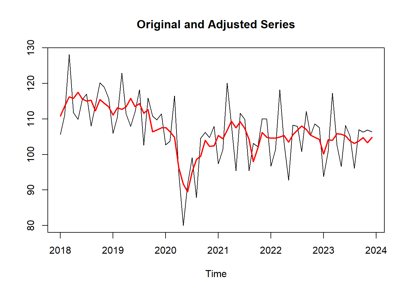

summary(sa)


Call:
seas(x = iip_nsa, x11 = "")

Coefficients:
                  Estimate Std. Error z value             Pr(>|z|)    
Leap Year           1.3553     2.2302   0.608               0.5434    
Weekday             0.4795     0.0707   6.783      0.0000000000118 ***
AR-Nonseasonal-01   0.7637     0.1694   4.507      0.0000065622008 ***
AR-Nonseasonal-02   0.1497     0.1352   1.108               0.2680    
AR-Nonseasonal-03  -0.2200     0.1111  -1.980               0.0477 *  
MA-Nonseasonal-01   0.8411     0.1498   5.615      0.0000000196736 ***
MA-Seasonal-12      0.9872     0.1184   8.339 < 0.0000000000000002 ***
---
Signif. codes:  0 '***' 0.001 '**' 0.01 '*' 0.05 '.' 0.1 ' ' 1

X11 adj.  ARIMA: (3 1 1)(0 1 1)  Obs.: 72  Transform: none
AICc: 329.5, BIC: 343.3  QS (no seasonality in final):    0  
Box-Ljung (no autocorr.): 31.82   Shapiro (normality): 0.9709 .

sa$model

regression{
  variables = td1coef
  b = (1.355331048 0.4795307604)
}

arima{
  model = (3 1 1)(0 1 1)
  ar = (0.7636725326 0.1497353889 -0.2200031053)
  ma = (0.8411102719 0.9872440861)
}

Tip

SEATS、X11どちらを選択しても事前調整済み系列の作成は REGARIMA によるため回帰の結果は同一となる。
参照: https://opac.ll.chiba-u.jp/da/curator/900119389/09127216_30_4_1-42.pdf

sa$fivebestmdl[1:8] %>%
    paste0(collapse = "") %>%
    paste0("</p>") %>%
    cat()

Best Five ARIMA Models

ARIMAモデルを(1 0 0)(0 1 1)とする。

sa <- seas(x = iip_nsa, x11 = "", arima.model = "(1 0 0)(0 1 1)")
summary(sa)


Call:
seas(x = iip_nsa, x11 = "", arima.model = "(1 0 0)(0 1 1)")

Coefficients:
                  Estimate Std. Error z value             Pr(>|z|)    
Leap Year          1.39985    2.29569   0.610                0.542    
Weekday            0.48286    0.07753   6.228 0.000000000472239299 ***
AR-Nonseasonal-01  0.89610    0.05002  17.913 < 0.0000000000000002 ***
MA-Seasonal-12     0.87881    0.10720   8.198 0.000000000000000244 ***
---
Signif. codes:  0 '***' 0.001 '**' 0.01 '*' 0.05 '.' 0.1 ' ' 1

X11 adj.  ARIMA: (1 0 0)(0 1 1)  Obs.: 72  Transform: none
AICc: 327.8, BIC: 337.2  QS (no seasonality in final):    0  
Box-Ljung (no autocorr.): 37.03 * Shapiro (normality): 0.974

sa$model

regression{
  variables = td1coef
  b = (1.399845881 0.4828605803)
}

arima{
  model = (1 0 0)(0 1 1)
  ar = 0.8960968219
  ma = 0.8788061537
}

経済産業省が公表している鉱工業生産指数の季節調整値(IIP_SA)とSEATSの結果およびX11の結果を比較する。

sa_seats <- seas(x = iip_nsa, arima.model = "(1 0 0)(0 1 1)") %>%
    data.frame() %>%
    {
        .[, c("date", "final")]
    } %>%
    {
        .$MA <- "SEATS"
        .
    }
sa_x11 <- seas(x = iip_nsa, arima.model = "(1 0 0)(0 1 1)", x11 = "", ) %>%
    data.frame() %>%
    {
        .[, c("date", "final")]
    } %>%
    {
        .$MA <- "X11"
        .
    }
sa_iip <- df_iip[, c("date", "IIP_SA")] %>%
    {
        .$MA <- "IIP_SA"
        colnames(.)[2] <- "final"
        .
    }
Reduce(function(x, y) rbind(x, y), list(sa_seats, sa_x11, sa_iip)) %>%
    ggplot(mapping = aes(x = date, y = final, col = MA, shape = MA)) + geom_line() + geom_point()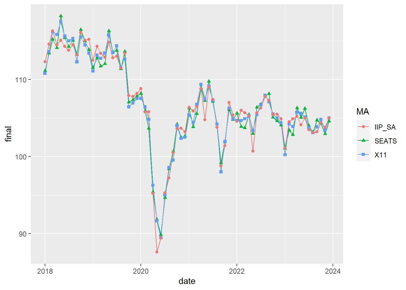

Tip

回帰変数に lpyear のみを指定すると以下のエラーメッセージが表示される。なお、エラーメッセージ中の for の後にはspcファイルのパス(Tempフォルダ)が続く。

seas(x = iip_nsa, regression.variables = "lpyear")

Error: X-13 run failed

Errors:
- Leap Year is already in the regression. Program error(s) halt execution for

祝日変数

2020年基準鉱工業指数に適用されている祝日変数を利用する。
スペックファイルで季節調整を乗法型と指定している鉱工業指数と合わせ、対数変換を行う。以降、同様。
出所: https://www.meti.go.jp/statistics/tyo/iip/pdf/b2020_kaitei_gaiyo.pdf

Tip

祝祭日調整に用いる祝日変数の作成方法については、以下のとおり。

季節指数計算の対象年月(12 年間)について、各年におけるそれぞれの月における平日(月曜日から金曜日)が祝日になる日数(A)を数え、次に1月から12月それぞれにおける12年間の祝日の平均値(B)を求めた後、各年におけるそれぞれの月の祝日日数(A)から平均値(B)を差し引いた値を用いる。
出所: https://www.meti.go.jp/statistics/tyo/iip/pdf/b2020_kaitei_gaiyo.pdf

xreg_holiday

        Jan    Feb    Mar    Apr    May    Jun    Jul    Aug    Sep    Oct
2011 -0.833 -0.083  0.167  0.000  0.250  0.000 -0.167 -0.500  0.083  0.083
2012  0.167 -1.083  0.167  0.000 -0.750  0.000 -0.167 -0.500 -0.917  0.083
2013  0.167 -0.083  0.167  0.000 -0.750  0.000 -0.167 -0.500  0.083  0.083
2014  0.167 -0.083  0.167  0.000 -0.750  0.000 -0.167 -0.500  0.083  0.083
2015  0.167 -0.083 -0.833  0.000  0.250  0.000 -0.167 -0.500  1.083  0.083
2016  0.167 -0.083  0.167  0.000  0.250  0.000 -0.167  0.500  0.083  0.083
2017  0.167 -1.083  0.167 -1.000  0.250  0.000 -0.167  0.500 -0.917  0.083
2018  0.167 -0.083  0.167  0.000 -0.750  0.000 -0.167 -0.500  0.083  0.083
2019  0.167 -0.083  0.167  1.000  1.250  0.000 -0.167  0.500  0.083  1.083
2020  0.167  0.917  0.167  0.000  0.250  0.000  0.833  0.500  0.083 -0.917
2021  0.167  0.917 -0.833  0.000  0.250  0.000  0.833  0.500  0.083 -0.917
2022 -0.833  0.917  0.167  0.000  0.250  0.000 -0.167  0.500  0.083  0.083
2023  0.167 -0.083  0.167 -1.000  0.250  0.000 -0.167  0.500 -0.917  0.083
2024  0.167  0.917  0.167  0.000 -0.750  0.000 -0.167  0.500  0.083  0.083
        Nov    Dec
2011  0.333  0.417
2012 -0.667  0.417
2013 -0.667  0.417
2014  0.333  0.417
2015  0.333  0.417
2016  0.333  0.417
2017  0.333 -0.583
2018 -0.667  0.417
2019 -0.667 -0.583
2020  0.333 -0.583
2021  0.333 -0.583
2022  0.333 -0.583
2023  0.333 -0.583
2024 -0.667 -0.583

Caution

regression.usertype を holiday とする。
「Usually, you want the holiday effect to be removed from the final series, so you need to specify regression.usertype = “holiday”. (The default is to include user defined variables in the final series.)」
出所: https://cran.r-project.org/web/packages/seasonal/seasonal.pdf

sa_x11_holiday <- seas(x = iip_nsa, x11 = "", transform.function = "log", x11.mode = "mult", xreg = xreg_holiday, regression.usertype = "holiday")

sa_x11_holiday %>%
    plot()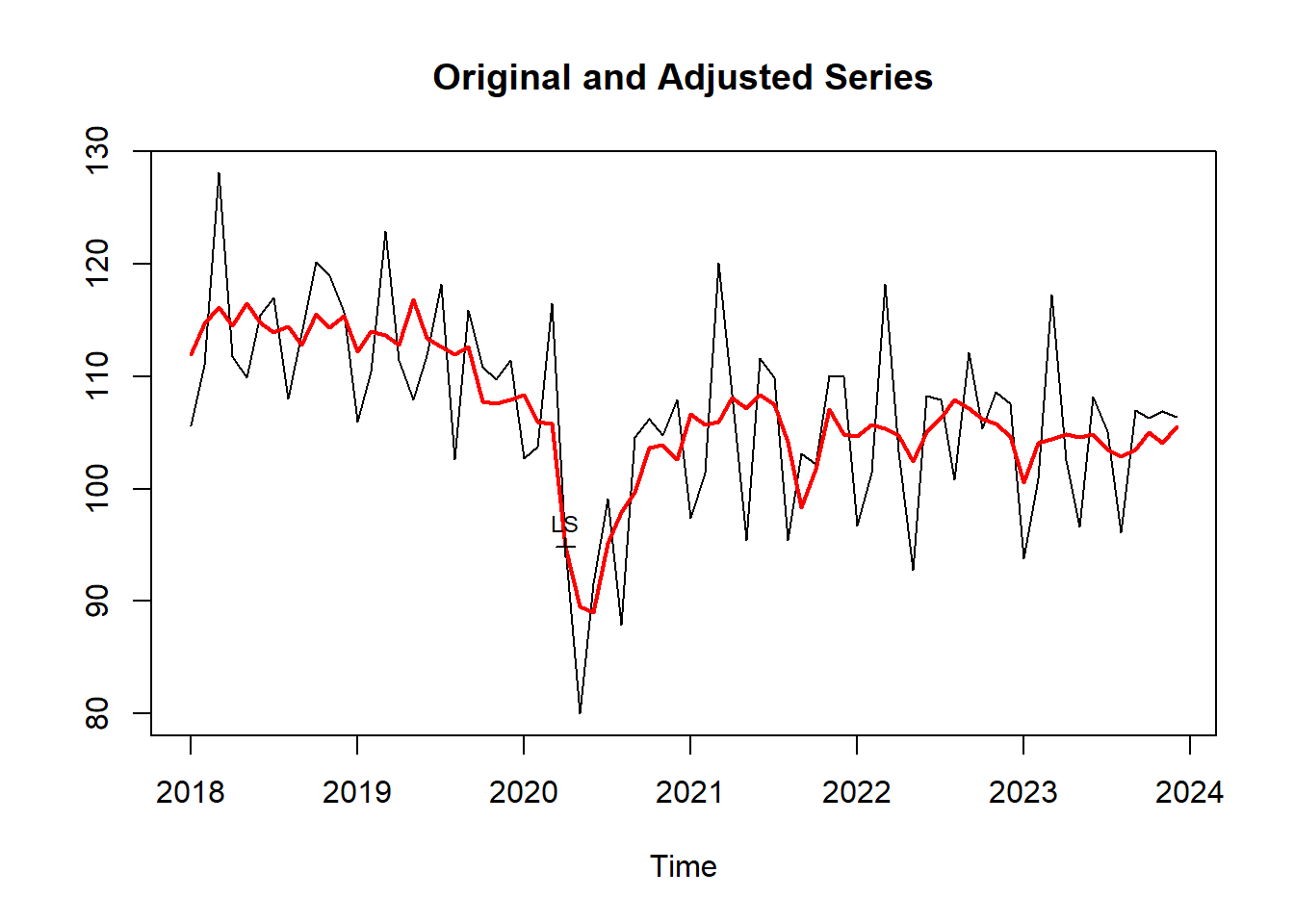

summary(sa_x11_holiday)


Call:
seas(x = iip_nsa, xreg = xreg_holiday, transform.function = "log", 
    x11 = "", x11.mode = "mult", regression.usertype = "holiday")

Coefficients:
                    Estimate Std. Error z value            Pr(>|z|)    
xreg              -0.0097753  0.0046864  -2.086               0.037 *  
Weekday            0.0056723  0.0007199   7.879 0.00000000000000329 ***
LS2020.Apr        -0.1206140  0.0269014  -4.484 0.00000734116067634 ***
MA-Nonseasonal-01  0.1526222  0.1069457   1.427               0.154    
MA-Seasonal-12     0.9988016  0.1266074   7.889 0.00000000000000305 ***
---
Signif. codes:  0 '***' 0.001 '**' 0.01 '*' 0.05 '.' 0.1 ' ' 1

X11 adj.  ARIMA: (0 1 1)(0 1 1)  Obs.: 72  Transform: log
AICc: 314.8, BIC: 325.6  QS (no seasonality in final):0.03806  
Box-Ljung (no autocorr.): 44.09 ** Shapiro (normality): 0.9854

sa_x11_holiday$model

regression{
  variables = (td1coef ls2020.Apr)
  user = xreg
  start = 2018.Jan
  data = (0.167 -0.083 0.167 0 -0.75 0 -0.167 -0.5 0.083 0.083 -0.667 0.417 0.167 -0.083 0.167 1 1.25 0 -0.167 0.5 0.083
  1.083 -0.667 -0.583 0.167 0.917 0.167 0 0.25 0 0.833 0.5 0.083 -0.917 0.333 -0.583 0.167 0.917 -0.833 0 0.25 0
  0.833 0.5 0.083 -0.917 0.333 -0.583 -0.833 0.917 0.167 0 0.25 0 -0.167 0.5 0.083 0.083 0.333 -0.583 0.167 -0.083
  0.167 -1 0.25 0 -0.167 0.5 -0.917 0.083 0.333 -0.583 0.167 0.917 0.167 0 -0.75 0 -0.167 0.5 0.083 0.083 -0.667
  -0.583)
  usertype = holiday
  b = (-0.009775331669 0.005672339937 -0.1206139572)
}

arima{
  model = (0 1 1)(0 1 1)
  ma = (0.1526222204 0.9988015939)
}

2020年4月の数値が異常値(LS(Level Shift，水準変化)として有意な説明変数(LS2020.Apr)に加えられている。同年月は新型コロナ禍により業況が悪化した時期である。

Tip

X-13ARIMA-SEATSで指定できる異常値は以下の6つ。

AO (Additive Outlier，加法的外れ値)
LS (Level Shift，水準変化)
TC (Temporary Change，一時的変化)
RP (Ramp，傾斜的変化)
TL (Temporary Level Shift, 一時的レベルシフト)
SO (Seasonal Outlier，季節性外れ値)

そのうち、RP、TL、SOはマニュアルで設定する必要がある。

出所:

Tip

異常値を説明変数としない場合は以下の方法による。

# outlier.types を 'none' とする。
seas(x = iip_nsa, x11 = "", transform.function = "log", x11.mode = "mult", xreg = xreg_holiday, regression.usertype = "holiday", outlier.types = "none") %>%
    summary()


Call:
seas(x = iip_nsa, xreg = xreg_holiday, transform.function = "log", 
    x11 = "", x11.mode = "mult", regression.usertype = "holiday", 
    outlier.types = "none")

Coefficients:
                    Estimate Std. Error z value             Pr(>|z|)    
xreg              -0.0094246  0.0047904  -1.967               0.0491 *  
Weekday            0.0053744  0.0007067   7.605 0.000000000000028411 ***
AR-Nonseasonal-01  0.9045956  0.1238288   7.305 0.000000000000276832 ***
AR-Nonseasonal-02 -0.0103306  0.1472428  -0.070               0.9441    
AR-Nonseasonal-03 -0.1041234  0.1122226  -0.928               0.3535    
MA-Nonseasonal-01  0.9208363  0.0715228  12.875 < 0.0000000000000002 ***
MA-Seasonal-12     0.9955995  0.1226343   8.118 0.000000000000000472 ***
---
Signif. codes:  0 '***' 0.001 '**' 0.01 '*' 0.05 '.' 0.1 ' ' 1

X11 adj.  ARIMA: (3 1 1)(0 1 1)  Obs.: 72  Transform: log
AICc: 333.1, BIC: 346.8  QS (no seasonality in final):0.00262  
Box-Ljung (no autocorr.): 37.01 * Shapiro (normality): 0.9618 *

祝日変数を加えない場合と比較する。

sa_x11_holiday <- seas(x = iip_nsa, x11 = "", transform.function = "log", x11.mode = "mult", regression.usertype = "holiday", xreg = xreg_holiday)
sa_x11 <- seas(x = iip_nsa, x11 = "", transform.function = "log")

# 祝日変数を加える場合
sa_x11_holiday$data[, "final"]

           Jan       Feb       Mar       Apr       May       Jun       Jul
2018 111.92600 114.68961 116.10976 114.52606 116.51286 114.80724 113.90585
2019 112.17400 114.03756 113.70553 112.84547 116.86861 113.37785 112.65659
2020 108.36134 105.92886 105.81370  94.84551  89.56224  89.04469  95.16746
2021 106.63680 105.72433 105.92885 108.09641 107.18578 108.39385 107.46500
2022 104.69168 105.72699 105.33594 104.74813 102.42440 104.97751 106.33672
2023 100.58587 104.09903 104.43746 104.83104 104.62112 104.84753 103.47962
           Aug       Sep       Oct       Nov       Dec
2018 114.41337 112.78876 115.56996 114.35340 115.40681
2019 111.95050 112.64836 107.79167 107.59688 107.94129
2020  97.87907  99.67701 103.63844 103.93828 102.62711
2021 104.12369  98.38007 101.78868 107.11081 104.85151
2022 107.93589 107.15410 106.19052 105.74602 104.65350
2023 102.85893 103.51903 104.97694 104.10680 105.55863

# 祝日変数を加えない場合
sa_x11$data[, "final"]

           Jan       Feb       Mar       Apr       May       Jun       Jul
2018 111.54134 114.65567 115.29644 114.40903 120.24186 114.75797 114.19865
2019 111.77431 114.11385 112.75360 111.77548 118.11796 113.15860 113.13099
2020 107.95239 105.00283 105.10101  94.85061  90.89392  89.11849  94.69289
2021 105.91141 105.04469 106.45463 108.09213 108.40196 108.50463 106.83711
2022 104.98321 105.14542 104.91270 104.60015 103.31046 105.11903 106.67995
2023  99.98770 104.58642 104.11551 105.56733 105.42752 104.99825 103.81013
           Aug       Sep       Oct       Nov       Dec
2018 115.23537 112.30130 115.66835 114.49435 114.10219
2019 111.54635 112.31336 106.79662 107.63815 107.91572
2020  97.50479  99.45273 104.55204 103.09261 102.67633
2021 103.93563  98.08898 102.58616 106.53031 104.83871
2022 107.98039 106.79780 105.93994 105.29270 104.48759
2023 102.89955 104.06660 104.84043 103.72956 105.29618

# 両者の差
sa_x11_holiday$data[, "final"] - sa_x11$data[, "final"]

              Jan          Feb          Mar          Apr          May
2018  0.384658442  0.033944369  0.813323809  0.117028735 -3.728999227
2019  0.399693663 -0.076296903  0.951933625  1.069986029 -1.249342180
2020  0.408949425  0.926029081  0.712696244 -0.005093748 -1.331676393
2021  0.725384728  0.679637407 -0.525773720  0.004278388 -1.216178438
2022 -0.291530010  0.581569254  0.423237848  0.147981544 -0.886062815
2023  0.598171252 -0.487389436  0.321949076 -0.736291734 -0.806403990
              Jun          Jul          Aug          Sep          Oct
2018  0.049275629 -0.292801337 -0.821999678  0.487458198 -0.098390298
2019  0.219248623 -0.474402390  0.404148187  0.334996705  0.995050307
2020 -0.073794932  0.474566377  0.374278327  0.224274300 -0.913593099
2021 -0.110779312  0.627884793  0.188059747  0.291098687 -0.797481890
2022 -0.141516948 -0.343236498 -0.044495504  0.356305329  0.250586190
2023 -0.150720436 -0.330508066 -0.040613991 -0.547565987  0.136504034
              Nov          Dec
2018 -0.140951021  1.304618477
2019 -0.041264414  0.025569269
2020  0.845673507 -0.049221901
2021  0.580498409  0.012803716
2022  0.453317928  0.165909442
2023  0.377234830  0.262451576

ゴールデンウィークで操業日が減少する影響でしょうか、5月は毎年に渡って祝日を加えない場合の方が季節調整値が大きく出ており、かつその差の平均値も他の月と比較すると大きいようです。

移動平均項数

季節変動成分

Tip

X11の季節変動成分移動平均項数の指定方法

エラーメッセージによるとs3x1, s3x3, s3x5, s3x9, s3x15, stable, msr, or x11default から選択する。

seas(x = iip_nsa, x11 = "", transform.function = "log", x11.mode = "mult", xreg = xreg_holiday, regression.usertype = "holiday", x11.seasonalma = "dummy")

Error: X-13 run failed

Errors: - Improper value(s) entered for seasonalma. Valid choices of seasonal filter are s3x1, s3x3, s3x5, s3x9, s3x15, stable, msr, or x11default.

鉱工業指数の季節調整法に合わせて移動平均項数は x11default とする。
季節調整法の適用状況（令和5年4月1日現在）: https://www.soumu.go.jp/main_content/000932400.xlsx
「These seasonal moving averages are n m moving averages, meaning that an n-term simple average is taken of a sequence of consecutive m-term simple averages」
その他参考資料
1. https://opac.ll.chiba-u.jp/da/curator/900020797/KJ00000171378.pdf
2. https://www.imes.boj.or.jp/research/papers/japanese/kk15-2-5.pdf

sa_x11_holiday_ma_default <- seas(x = iip_nsa, x11 = "", transform.function = "log", x11.mode = "mult", xreg = xreg_holiday, regression.usertype = "holiday", x11.seasonalma = "x11default")

summary(sa_x11_holiday_ma_default)


Call:
seas(x = iip_nsa, xreg = xreg_holiday, transform.function = "log", 
    x11 = "", x11.mode = "mult", regression.usertype = "holiday", 
    x11.seasonalma = "x11default")

Coefficients:
                    Estimate Std. Error z value            Pr(>|z|)    
xreg              -0.0097753  0.0046864  -2.086               0.037 *  
Weekday            0.0056723  0.0007199   7.879 0.00000000000000329 ***
LS2020.Apr        -0.1206140  0.0269014  -4.484 0.00000734116067634 ***
MA-Nonseasonal-01  0.1526222  0.1069457   1.427               0.154    
MA-Seasonal-12     0.9988016  0.1266074   7.889 0.00000000000000305 ***
---
Signif. codes:  0 '***' 0.001 '**' 0.01 '*' 0.05 '.' 0.1 ' ' 1

X11 adj.  ARIMA: (0 1 1)(0 1 1)  Obs.: 72  Transform: log
AICc: 314.8, BIC: 325.6  QS (no seasonality in final):0.03806  
Box-Ljung (no autocorr.): 44.09 ** Shapiro (normality): 0.9854

sa_x11_holiday_ma_default$model

regression{
  variables = (td1coef ls2020.Apr)
  user = xreg
  start = 2018.Jan
  data = (0.167 -0.083 0.167 0 -0.75 0 -0.167 -0.5 0.083 0.083 -0.667 0.417 0.167 -0.083 0.167 1 1.25 0 -0.167 0.5 0.083
  1.083 -0.667 -0.583 0.167 0.917 0.167 0 0.25 0 0.833 0.5 0.083 -0.917 0.333 -0.583 0.167 0.917 -0.833 0 0.25 0
  0.833 0.5 0.083 -0.917 0.333 -0.583 -0.833 0.917 0.167 0 0.25 0 -0.167 0.5 0.083 0.083 0.333 -0.583 0.167 -0.083
  0.167 -1 0.25 0 -0.167 0.5 -0.917 0.083 0.333 -0.583 0.167 0.917 0.167 0 -0.75 0 -0.167 0.5 0.083 0.083 -0.667
  -0.583)
  usertype = holiday
  b = (-0.009775331669 0.005672339937 -0.1206139572)
}

arima{
  model = (0 1 1)(0 1 1)
  ma = (0.1526222204 0.9988015939)
}

sa_x11_holiday_ma_default$data[, "final"]

           Jan       Feb       Mar       Apr       May       Jun       Jul
2018 111.92600 114.68961 116.10976 114.52606 116.51286 114.80724 113.90585
2019 112.17400 114.03756 113.70553 112.84547 116.86861 113.37785 112.65659
2020 108.36134 105.92886 105.81370  94.84551  89.56224  89.04469  95.16746
2021 106.63680 105.72433 105.92885 108.09641 107.18578 108.39385 107.46500
2022 104.69168 105.72699 105.33594 104.74813 102.42440 104.97751 106.33672
2023 100.58587 104.09903 104.43746 104.83104 104.62112 104.84753 103.47962
           Aug       Sep       Oct       Nov       Dec
2018 114.41337 112.78876 115.56996 114.35340 115.40681
2019 111.95050 112.64836 107.79167 107.59688 107.94129
2020  97.87907  99.67701 103.63844 103.93828 102.62711
2021 104.12369  98.38007 101.78868 107.11081 104.85151
2022 107.93589 107.15410 106.19052 105.74602 104.65350
2023 102.85893 103.51903 104.97694 104.10680 105.55863

参考としてs3x15とした場合。

sa_x11_holiday_ma_3_15 <- seas(x = iip_nsa, x11 = "", transform.function = "log", x11.mode = "mult", xreg = xreg_holiday, regression.usertype = "holiday", x11.seasonalma = "s3x15")
sa_x11_holiday_ma_3_15$data[, "final"]

           Jan       Feb       Mar       Apr       May       Jun       Jul
2018 111.79621 114.41905 116.02374 113.67072 117.87946 114.46810 113.38043
2019 112.21968 113.80057 113.54598 112.12830 118.01919 113.12399 112.29168
2020 108.72605 105.71051 105.51730  94.49156  90.16128  88.99710  95.07124
2021 107.29176 105.55011 105.60227 108.04731 107.51733 108.42878 107.54626
2022 105.48447 105.55011 104.95257 105.02849 102.53118 105.22255 106.65859
2023 101.29503 104.00795 104.15344 105.27068 104.63162 105.12539 103.89080
           Aug       Sep       Oct       Nov       Dec
2018 114.39723 113.12633 115.91457 114.48920 115.42858
2019 111.94549 112.94909 107.89932 107.65800 107.89409
2020  97.82959  99.93299 103.45103 103.85953 102.44996
2021 104.08967  98.49991 101.55080 106.96710 104.44389
2022 107.81958 107.09835 105.75927 105.50979 104.21368
2023 102.79228 103.26133 104.56563 103.85816 105.11779

cbind(sa_x11_holiday_ma_default$data[, "final"], sa_x11_holiday_ma_3_15$data[, "final"]) %>%
    {
        date = as.Date(.)
        data.frame(date, ., check.names = F)
    } %>%
    gather(key = "key", value = "value", colnames(.)[-1]) %>%
    ggplot(mapping = aes(x = date, y = value, col = key)) + geom_point() + geom_line() + theme(legend.position = "top", legend.title = element_blank())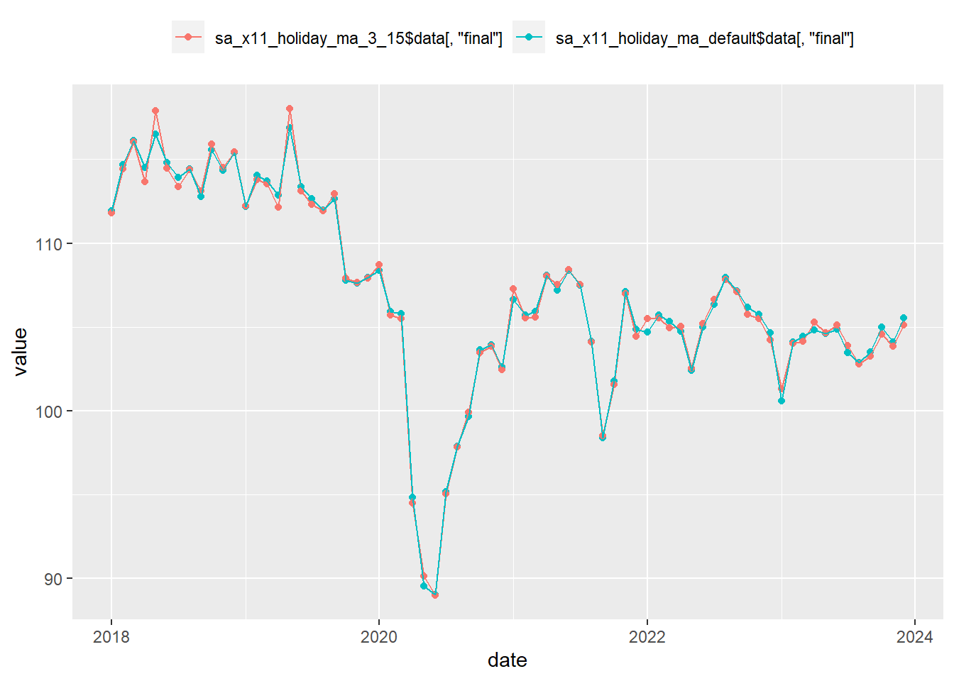

趨勢循環変動成分

Tip

X11の趨勢循環変動成分移動平均項数の指定方法

ヘンダーソン加重移動平均による。
指定項数は奇数とする必要がある。

seas(x = iip_nsa, x11 = "", transform.function = "log", x11.mode = "mult", xreg = xreg_holiday, regression.usertype = "holiday", x11.seasonalma = "x11default", x11.trendma = 1000)

Error: X-13 run failed

Errors: - Length of Henderson trend filter must be a positive odd integer.

エラーメッセージによると最大指定項数は101。

seas(x = iip_nsa, x11 = "", transform.function = "log", x11.mode = "mult", xreg = xreg_holiday, regression.usertype = "holiday", x11.seasonalma = "x11default", x11.trendma = 11111)

Error: X-13 run failed

Errors: - Length of Henderson filter cannot exceed 101. No seasonal adjustment this run

Tip

「趨勢循環変動成分をヘンダーソン加重移動平均による算出する際の移動平均項数を指定。省略時には、月次データの場合、通常は13項移動平均が適用されますが、著しく不規則変動の大きい系列には、23項移動平均を、また非常に滑らかな系列については、9項移動平均が適用されます。四半期データの場合は、5項移動平均、または7項移動平均が適用されます」

出所: https://www.boj.or.jp/statistics/outline/ref/ron9702c.htm

移動平均項数を9、23とした場合と指定せずにデフォルトとした場合とを比較する。

date <- df_iip$date
ma9 <- seas(x = iip_nsa, x11 = "", transform.function = "log", x11.mode = "mult", xreg = xreg_holiday, regression.usertype = "holiday", x11.seasonalma = "x11default", x11.trendma = 9) %>%
    {
        .$data[, "final"]
    }
ma23 <- seas(x = iip_nsa, x11 = "", transform.function = "log", x11.mode = "mult", xreg = xreg_holiday, regression.usertype = "holiday", x11.seasonalma = "x11default", x11.trendma = 23) %>%
    {
        .$data[, "final"]
    }
madefault <- seas(x = iip_nsa, x11 = "", transform.function = "log", x11.mode = "mult", xreg = xreg_holiday, regression.usertype = "holiday", x11.seasonalma = "x11default") %>%
    {
        .$data[, "final"]
    }
data.frame(ma9, ma23) %>%
    data.frame(date, ., madefault) %>%
    gather(key = "key", value = "value", colnames(.)[-1]) %>%
    ggplot(mapping = aes(x = date, y = value, col = key, shape = key)) + geom_line() + geom_point()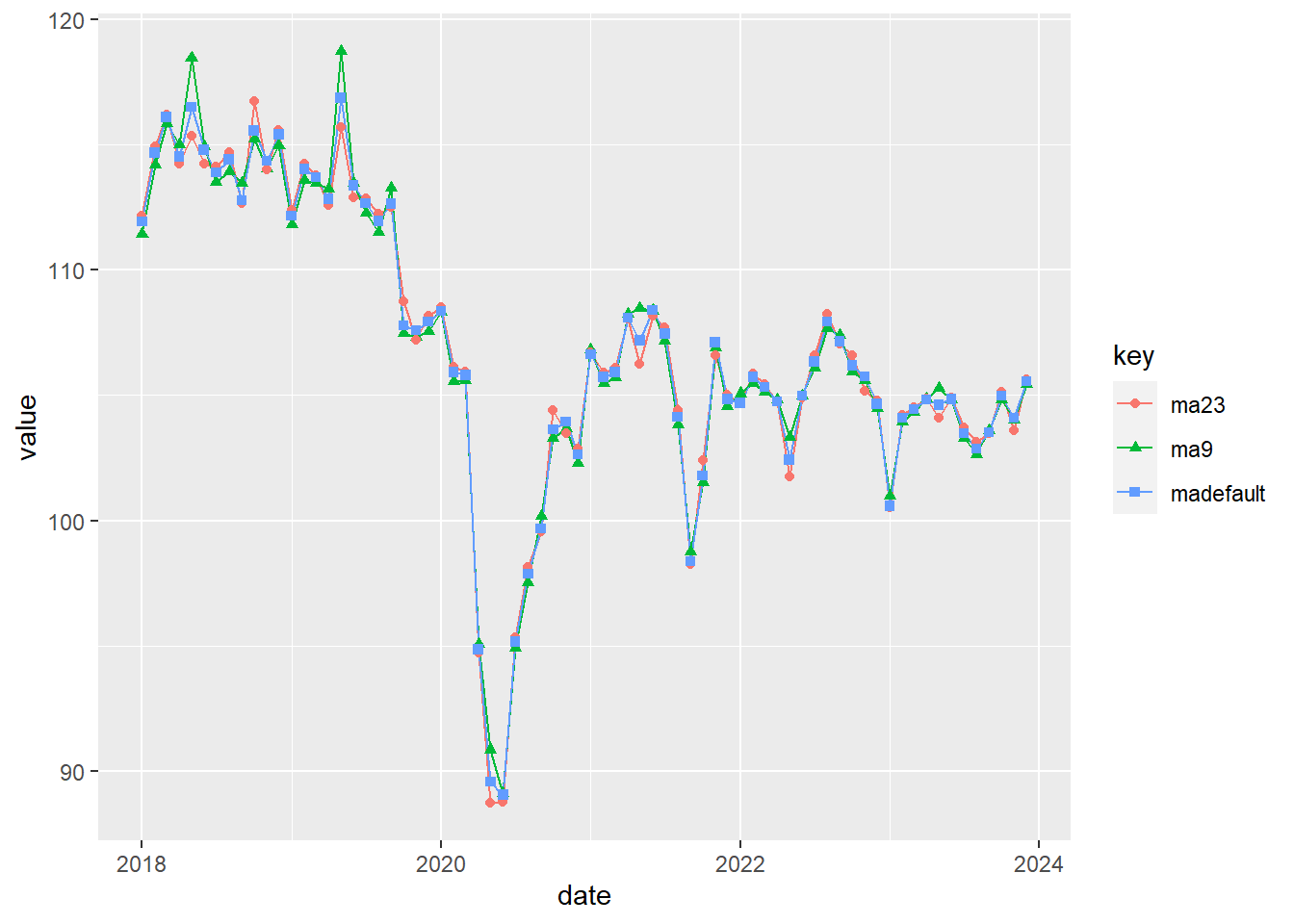

特異項の管理限界

Tip

「異常値管理限界（判定基準）の上限および下限を指定。判定基準から異常値として判定された不規則変動成分に偏りの大きさに応じた修正ウエイトをかけて、「異常値調整済不規則変動成分」を算出する。省略時は、上限2.5、下限1.5が設定されます」

出所: https://www.boj.or.jp/statistics/outline/ref/ron9702c.htm

Tip

鉱工業指数の季節調整法の管理限界設定はデフォルト(上限2.5、下限1.5)。

出所:季節調整法の適用状況（令和5年4月1日現在）: https://www.soumu.go.jp/main_content/000932400.xlsx

sigmalim_0.5_4.5 <- seas(x = iip_nsa, x11 = "", transform.function = "log", x11.mode = "mult", xreg = xreg_holiday, regression.usertype = "holiday", x11.seasonalma = "x11default", x11.sigmalim = c(0.5, 4.5))  # c(下限,上限)
sigmalim_1.5_2.5 <- seas(x = iip_nsa, x11 = "", transform.function = "log", x11.mode = "mult", xreg = xreg_holiday, regression.usertype = "holiday", x11.seasonalma = "x11default", x11.sigmalim = c(1.5, 2.5))
cbind(sigmalim_0.5_4.5$data[, "final"], sigmalim_1.5_2.5$data[, "final"]) %>%
    {
        date = as.Date(.)
        add_column(.data = data.frame(., check.names = F), date, .before = 1)
    } %>%
    gather(key = "key", value = "value", colnames(.)[-1]) %>%
    ggplot(mapping = aes(x = date, y = value, col = key)) + geom_line() + geom_point()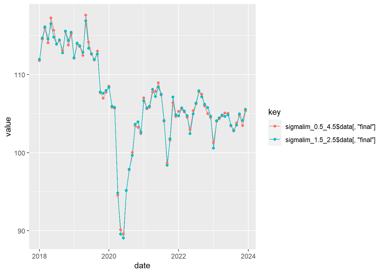

Tip

指定しない場合はデフォルトが設定される。

# 指定あり
seas(x = iip_nsa, x11 = "", transform.function = "log", x11.mode = "mult", xreg = xreg_holiday, regression.usertype = "holiday", x11.seasonalma = "x11default", x11.sigmalim = c(1.5, 2.5)) %>%
    {
        .$data[, "final"]
    }
# 指定なし
seas(x = iip_nsa, x11 = "", transform.function = "log", x11.mode = "mult", xreg = xreg_holiday, regression.usertype = "holiday", x11.seasonalma = "x11default") %>%
    {
        .$data[, "final"]
    }

           Jan       Feb       Mar       Apr       May       Jun       Jul
2018 111.92600 114.68961 116.10976 114.52606 116.51286 114.80724 113.90585
2019 112.17400 114.03756 113.70553 112.84547 116.86861 113.37785 112.65659
2020 108.36134 105.92886 105.81370  94.84551  89.56224  89.04469  95.16746
2021 106.63680 105.72433 105.92885 108.09641 107.18578 108.39385 107.46500
2022 104.69168 105.72699 105.33594 104.74813 102.42440 104.97751 106.33672
2023 100.58587 104.09903 104.43746 104.83104 104.62112 104.84753 103.47962
           Aug       Sep       Oct       Nov       Dec
2018 114.41337 112.78876 115.56996 114.35340 115.40681
2019 111.95050 112.64836 107.79167 107.59688 107.94129
2020  97.87907  99.67701 103.63844 103.93828 102.62711
2021 104.12369  98.38007 101.78868 107.11081 104.85151
2022 107.93589 107.15410 106.19052 105.74602 104.65350
2023 102.85893 103.51903 104.97694 104.10680 105.55863
           Jan       Feb       Mar       Apr       May       Jun       Jul
2018 111.92600 114.68961 116.10976 114.52606 116.51286 114.80724 113.90585
2019 112.17400 114.03756 113.70553 112.84547 116.86861 113.37785 112.65659
2020 108.36134 105.92886 105.81370  94.84551  89.56224  89.04469  95.16746
2021 106.63680 105.72433 105.92885 108.09641 107.18578 108.39385 107.46500
2022 104.69168 105.72699 105.33594 104.74813 102.42440 104.97751 106.33672
2023 100.58587 104.09903 104.43746 104.83104 104.62112 104.84753 103.47962
           Aug       Sep       Oct       Nov       Dec
2018 114.41337 112.78876 115.56996 114.35340 115.40681
2019 111.95050 112.64836 107.79167 107.59688 107.94129
2020  97.87907  99.67701 103.63844 103.93828 102.62711
2021 104.12369  98.38007 101.78868 107.11081 104.85151
2022 107.93589 107.15410 106.19052 105.74602 104.65350
2023 102.85893 103.51903 104.97694 104.10680 105.55863

予測期間

Tip

ARIMAモデルを用いて、4~5年分の予測値を推計します。原系列にこの予測値を追加した事前調整済原系列に対しX-11の移動平均を行うと、系列末端部分においても予測値を利用した中心移動平均による移動平均が可能となり、季調済系列の安定性が高まります。X-11の標準中心移動平均では、前後約7年分のデータを使用しますが、6、7年めのデータのウエイトはかなり小さいので、5年分程度のデータがあれば十分です。

出所: https://www.boj.or.jp/statistics/outline/ref/ron9702c.htm

Tip

鉱工業指数の先行き予測期間は12か月、後戻り予測期間はなし。

出所:季節調整法の適用状況（令和5年4月1日現在）: https://www.soumu.go.jp/main_content/000932400.xlsx

先行き予測期間を「12か月」とした場合と「なし」とした場合を比較します。

ma_maxback_0_maxlead_12 <- seas(x = iip_nsa, x11 = "", transform.function = "log", x11.mode = "mult", xreg = xreg_holiday, regression.usertype = "holiday", x11.seasonalma = "x11default", forecast.maxlead = 12, forecast.maxback = 0)
ma_maxback_0_maxlead_0 <- seas(x = iip_nsa, x11 = "", transform.function = "log", x11.mode = "mult", xreg = xreg_holiday, regression.usertype = "holiday", x11.seasonalma = "x11default", forecast.maxlead = 0, forecast.maxback = 0)
cbind(ma_maxback_0_maxlead_0$data[, "final"], ma_maxback_0_maxlead_12$data[, "final"]) %>%
    {
        date <- as.Date(.)
        add_column(.data = data.frame(., check.names = F), date, .before = 1)
    } %>%
    gather(key = "key", value = "value", colnames(.)[-1]) %>%
    ggplot(mapping = aes(x = date, y = value, col = key)) + geom_line() + geom_point()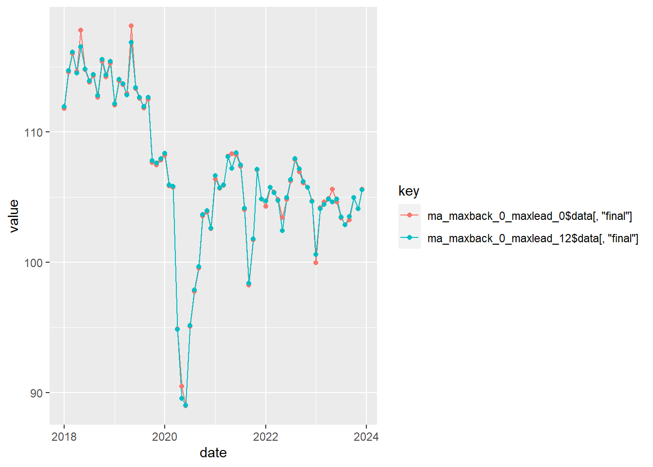

Tip

今回適用した祝日変数の範囲を超えているためエラーが出る。

seas(x = iip_nsa, x11 = "", transform.function = "log", x11.mode = "mult", xreg = xreg_holiday, regression.usertype = "holiday", x11.seasonalma = "x11default", forecast.maxlead = 13)

Error: X-13 run failed

Errors: - forecasts end date, 2025.Jan, must end on or before user-defined regression variables end date, 2024.Dec.

ARIMAモデルと曜日調整の選択

Tip

前回基準改定作業に則り、①（011）（011）モデルで仮外れ値を検出、②仮外れ値を変数として設定した上で、BICの小さいモデルを選ぶこととした。

平成27年基準における選択結果は、以下のとおり。

生産(110）（011）
出荷（011）（011）
在庫及び在庫率（010）（011）
稼働率（111）（011）
生産予測（110）（011）

出所: 季節調整法の適用状況（令和5年4月1日現在）: https://www.soumu.go.jp/main_content/000932400.xlsx

Tip

曜日はデフォルト、祝祭日はカレンダーよりユーザ型回帰変数を用い、左記のとおりRegARIMAモデルを決定。なお、うるう年が有意ではなかったため設定はしていない。異常値は、定期的（年間補正時）にoutlierコマンドによって全てのタイプの異常値を検出する。原則として検出された全ての異常値を取り入れるが、経済事象や系列の性質を考慮した上で、暫定季節指数の安定性に関する検証等を行い、異常値の検出期間の設定や、異常値のタイプ等を必要に応じて調整する。

出所: 季節調整法の適用状況（令和5年4月1日現在）: https://www.soumu.go.jp/main_content/000932400.xlsx

# 鉱工業生産指数の季節調整系列
iip_sa <- df_iip$IIP_SA %>%
    ts(start = df_iip$date %>%
        head(1) %>%
        {
            c(year(.), month(.))
        }, end = df_iip$date %>%
        tail(1) %>%
        {
            c(year(.), month(.))
        }, frequency = 12)
# seas {seasonal} を利用した季節調整
sa_by_seas <- seas(x = iip_nsa, x11 = "", transform.function = "log", x11.mode = "mult", xreg = xreg_holiday, regression.usertype = "holiday", x11.seasonalma = "x11default", forecast.maxlead = 12, forecast.maxback = 0, outlier.types = "all", regression.variables = c("td"), arima.model = "(1 1 0)(0 1 1)")
cbind(sa_by_seas$data[, "final"] %>%
    round(1), iip_sa) %>%
    {
        date <- as.Date(.)
        add_column(.data = data.frame(., check.names = F), date, .before = 1)
    } %>%
    gather(key = "key", value = "value", colnames(.)[-1]) %>%
    ggplot(mapping = aes(x = date, y = value, col = key)) + geom_line() + geom_point()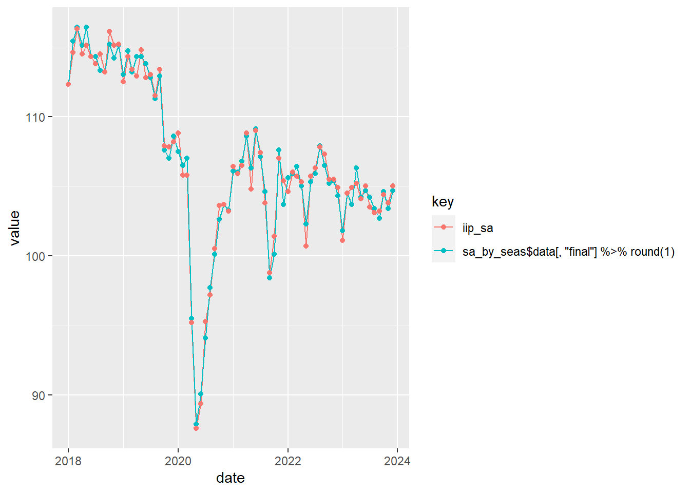

list(sa_by_seas = sa_by_seas$data[, "final"] %>%
    round(1), iip_sa = iip_sa)

$sa_by_seas
       Jan   Feb   Mar   Apr   May   Jun   Jul   Aug   Sep   Oct   Nov   Dec
2018 112.3 115.4 116.4 115.1 116.4 114.3 114.3 113.3 113.2 115.2 114.2 115.1
2019 113.0 114.7 113.2 114.3 114.3 113.8 112.8 111.3 112.9 107.6 107.0 108.6
2020 107.5 106.5 107.0  95.5  87.9  90.1  94.1  97.7 100.1 102.6 103.7 103.3
2021 106.1 106.0 106.8 108.6 106.3 109.1 107.1 104.6  98.4 100.1 107.6 103.7
2022 105.6 105.9 106.4 105.0 102.3 105.3 105.9 107.9 106.5 105.2 105.4 104.3
2023 101.8 104.5 103.7 106.3 104.2 104.7 104.2 103.4 102.7 104.6 103.4 104.7

$iip_sa
       Jan   Feb   Mar   Apr   May   Jun   Jul   Aug   Sep   Oct   Nov   Dec
2018 112.3 114.6 116.3 114.5 115.1 114.3 113.8 114.5 113.2 116.1 115.1 115.2
2019 112.5 114.3 113.4 112.9 114.8 112.8 113.0 111.5 113.4 107.9 107.8 108.2
2020 108.8 105.8 105.8  95.2  87.6  89.4  95.3  97.2 100.5 103.6 103.7 103.2
2021 106.4 105.9 106.5 108.8 104.8 109.0 107.4 103.8  98.8 101.4 107.0 105.4
2022 104.6 106.0 105.7 105.3 100.7 105.7 106.3 107.8 107.3 105.5 105.5 104.9
2023 101.1 104.5 104.9 105.2 104.1 105.0 103.5 103.1 103.2 104.4 103.8 105.0

sa_by_seas$model

regression{
  variables = (td ls2020.Apr tc2020.May tc2021.Sep)
  user = xreg
  start = 2018.Jan
  data = (0.167 -0.083 0.167 0 -0.75 0 -0.167 -0.5 0.083 0.083 -0.667 0.417 0.167 -0.083 0.167 1 1.25 0 -0.167 0.5 0.083
  1.083 -0.667 -0.583 0.167 0.917 0.167 0 0.25 0 0.833 0.5 0.083 -0.917 0.333 -0.583 0.167 0.917 -0.833 0 0.25 0
  0.833 0.5 0.083 -0.917 0.333 -0.583 -0.833 0.917 0.167 0 0.25 0 -0.167 0.5 0.083 0.083 0.333 -0.583 0.167 -0.083
  0.167 -1 0.25 0 -0.167 0.5 -0.917 0.083 0.333 -0.583 0.167 0.917 0.167 0 -0.75 0 -0.167 0.5 0.083 0.083 -0.667
  -0.583)
  usertype = holiday
  b = (-0.007691896234 0.004779864019 -0.002075744234 0.01062036089 0.0008772311586 0.01495507019 -0.01599901823
  -0.1043061562 -0.1011703923 -0.08235363489)
}

arima{
  model = (1 1 0)(0 1 1)
  ar = -0.4281277311
  ma = 0.9289627598
}

sa_by_seas %>%
    summary()


Call:
seas(x = iip_nsa, xreg = xreg_holiday, transform.function = "log", 
    x11 = "", x11.mode = "mult", regression.usertype = "holiday", 
    x11.seasonalma = "x11default", forecast.maxlead = 12, forecast.maxback = 0, 
    outlier.types = "all", regression.variables = c("td"), arima.model = "(1 1 0)(0 1 1)")

Coefficients:
                    Estimate Std. Error z value             Pr(>|z|)    
xreg              -0.0076919  0.0039438  -1.950             0.051131 .  
Mon                0.0047799  0.0051845   0.922             0.356551    
Tue               -0.0020757  0.0049689  -0.418             0.676134    
Wed                0.0106204  0.0049943   2.126             0.033463 *  
Thu                0.0008772  0.0049518   0.177             0.859388    
Fri                0.0149551  0.0048368   3.092             0.001989 ** 
Sat               -0.0159990  0.0045031  -3.553             0.000381 ***
LS2020.Apr        -0.1043062  0.0214225  -4.869           0.00000112 ***
TC2020.May        -0.1011704  0.0211747  -4.778           0.00000177 ***
TC2021.Sep        -0.0823536  0.0194004  -4.245           0.00002187 ***
AR-Nonseasonal-01 -0.4281277  0.1019111  -4.201           0.00002657 ***
MA-Seasonal-12     0.9289628  0.1107758   8.386 < 0.0000000000000002 ***
---
Signif. codes:  0 '***' 0.001 '**' 0.01 '*' 0.05 '.' 0.1 ' ' 1

X11 adj.  ARIMA: (1 1 0)(0 1 1)  Obs.: 72  Transform: log
AICc: 302.1, BIC:   321  QS (no seasonality in final):0.1736  
Box-Ljung (no autocorr.): 24.31   Shapiro (normality): 0.9815

plot(sa_by_seas)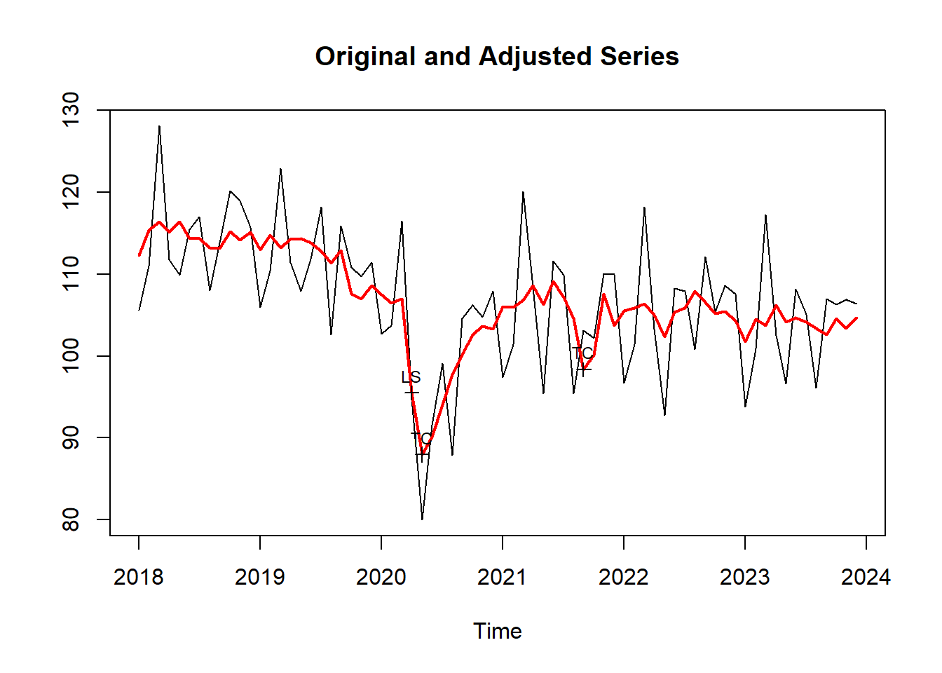

Tip

曜日変動の回帰変数の種類について
1. td
  - 月中の曜日構成の相違により引き起こされる変動及び閏年による変動を調整。曜日調整のための回帰変数は、以下の6つの変数がある。
    1. (月曜日の数) - (日曜日の数)
    2. (火曜日の数) - (日曜日の数)
    3. (水曜日の数) - (日曜日の数)
    4. (木曜日の数) - (日曜日の数)
    5. (金曜日の数) - (日曜日の数)
    6. (土曜日の数) - (日曜日の数)
2. tdnolpyear
  - 月中の曜日構成の相違により引き起こされる変動のみを調整し、閏年調整は行わない。
3. td1coef
  - 平日の数(月曜日から金曜日までの数)の相違により引き起こされる変動及び閏年による変動を調整。
4. lpyear
  - 閏年による変動のみを調整。
出所: https://www.mhlw.go.jp/content/10700000/001097961.pdf

Tip

d10
- 季節変動（曜日変動等も加えたもの）（S）
d11
- 季節調整済系列（TC･I）
d12
- 趨勢循環成分（TC）
d13
- 不規則変動成分（I）
d16
- 季節 × 曜日変動
出所: https://www.meti.go.jp/statistics/tyo/iip/riyou-4.pdf

最終更新

Sys.time()

[1] "2024-04-09 15:09:01 JST"

R、Quarto、Package

R.Version()$version.string

[1] "R version 4.3.3 (2024-02-29 ucrt)"

quarto::quarto_version()

[1] '1.4.542'

packageVersion(pkg = "tidyverse")

[1] '2.0.0'

著者

アセット･マネジメント･コンサルティング株式会社 https://www.am-consulting.co.jp
法人概要 https://www.contact.am-consulting.co.jp/company-brochure/
代表取締役三竹道雄 https://www.contact.am-consulting.co.jp/mitake-michio/
公開コンテンツリスト https://www.am-consulting.co.jp/amc-all-contents.html
Charts https://www.am-consulting.co.jp/charts.html
法令検索 https://www.laws.am-consulting.co.jp/
SaECaNet https://www.saecanet.com/
twitter https://twitter.com/amc_corporation
youtube https://www.youtube.com/user/michiomitake
twilog https://twilog.togetter.com/amc_corporation
github https://github.com/am-consulting