library(rstan)
library(dplyr)
rstan_options(auto_write = TRUE)
options(mc.cores = parallel::detectCores())
packageVersion("rstan")
[1] '2.32.6'Rでデータサイエンス
library(rstan)
library(dplyr)
rstan_options(auto_write = TRUE)
options(mc.cores = parallel::detectCores())
packageVersion("rstan")[1] '2.32.6'# sample data
N <- 50
m0 <- 10
G <- matrix(data = 1)
F <- matrix(data = 1)
# 正定値対称行列
C0 <- matrix(0.1)
W <- matrix(0.15) # 経時的変動なし
V <- matrix(0.2) # 経時的変動なし
# 観測値
x <- y <- matrix(ncol = N, nrow = 1)
x[1, 1] <- rnorm(n = 1, mean = m0, sd = sqrt(C0[1, 1]))
for (t in 2:N) {
x[1, t] <- rnorm(n = 1, mean = G[1, 1] %*% x[1, t - 1], sd = sqrt(W[1, 1]))
}
for (t in 1:N) {
y[1, t] <- rnorm(n = 1, mean = F[1, 1] %*% x[1, t], sd = sqrt(V[1, 1]))
}# stan code
model_code = "
data{
int<lower=1> N; // 時系列データの要素数
matrix[1,N] y; // 観測値
// 係数行列
matrix[1,1] G; // 状態遷移行列(状態発展行列,システム行列) (p × p)行列
matrix[1,1] F; // 観測行列 (1 × p)行列
// 事前分布
vector[1] m0; // 平均(p次元)ベクトル
cov_matrix[1] C0; // 分散,正定値対称行列 共分散行列 (p × p)行列
}
parameters{
// ノイズ 経時的変動なし
cov_matrix[1] W; // システムノイズの分散,正定値対称行列 共分散行列 (p × p)行列
cov_matrix[1] V; // 観測ノイズの分散,正定値対称行列
}
// よってWとVの事前分布は、指定しない場合のStanのデフォルトである、無情報事前分布となる。
model{
y ~ gaussian_dlm_obs(F,G,V,W,m0,C0);
// https://mc-stan.org/docs/2_28/functions-reference/gaussian-dynamic-linear-models.html
// 線形・ガウス型状態空間モデルの尤度を計算する関数
}
"# MCMC
dim(m0)
# Exception: mismatch in number dimensions declared and found in context;
# processing stage=data initialization;
# variable name=m0; dims declared=(1); dims found=()NULL# gaussian_dlm_obs()を利用する場合、ベクトルとはいっても要素数が1つの場合は次元を設定する必要がある。
# dim(m0) <- 1
# または
m0 <- as.array(m0)
dim(m0)[1] 1data_list <- list(N = N, y = y, G = G, F = t(F), m0 = m0, C0 = C0)
mcmc_result <- stan(model_code = model_code, data = data_list, refresh = 0)# パラメータの平均、標準偏差、信用区間、R hat の確認
print(mcmc_result)Inference for Stan model: anon_model.
4 chains, each with iter=2000; warmup=1000; thin=1;
post-warmup draws per chain=1000, total post-warmup draws=4000.
mean se_mean sd 2.5% 25% 50% 75% 97.5% n_eff Rhat
W[1,1] 0.19 0.00 0.09 0.08 0.13 0.18 0.23 0.41 1853 1
V[1,1] 0.24 0.00 0.08 0.11 0.19 0.23 0.29 0.43 2243 1
lp__ -10.15 0.02 0.97 -12.77 -10.57 -9.85 -9.45 -9.18 1645 1
Samples were drawn using NUTS(diag_e) at Tue Mar 12 13:40:24 2024.
For each parameter, n_eff is a crude measure of effective sample size,
and Rhat is the potential scale reduction factor on split chains (at
convergence, Rhat=1).mcmc_result %>%
str() %>%
capture.output() %>%
{
paste0(.[1:20], collapse = "\n")
} %>%
cat()Formal class 'stanfit' [package "rstan"] with 10 slots
..@ model_name: chr "anon_model"
..@ model_pars: chr [1:3] "W" "V" "lp__"
..@ par_dims :List of 3
.. ..$ W : num [1:2] 1 1
.. ..$ V : num [1:2] 1 1
.. ..$ lp__: num(0)
..@ mode : int 0
..@ sim :List of 12
.. ..$ samples :List of 4
.. .. ..$ :List of 3
.. .. .. ..$ W[1,1]: num [1:2000] 1.116 1.116 1.116 0.647 0.631 ...
.. .. .. ..$ V[1,1]: num [1:2000] 0.0421 0.0421 0.0421 0.0547 0.0528 ...
.. .. .. ..$ lp__ : num [1:2000] -19 -19 -19 -14.6 -14.6 ...
.. .. .. ..- attr(*, "test_grad")= logi FALSE
.. .. .. ..- attr(*, "args")=List of 16
.. .. .. .. ..$ append_samples : logi FALSE
.. .. .. .. ..$ chain_id : num 1
.. .. .. .. ..$ control :List of 12
.. .. .. .. .. ..$ adapt_delta : num 0.8mcmc_result@sim$samples[[1]] %>%
str() %>%
capture.output() %>%
{
paste0(.[1:20], collapse = "\n")
} %>%
cat()List of 3
$ W[1,1]: num [1:2000] 1.116 1.116 1.116 0.647 0.631 ...
$ V[1,1]: num [1:2000] 0.0421 0.0421 0.0421 0.0547 0.0528 ...
$ lp__ : num [1:2000] -19 -19 -19 -14.6 -14.6 ...
- attr(*, "test_grad")= logi FALSE
- attr(*, "args")=List of 16
..$ append_samples : logi FALSE
..$ chain_id : num 1
..$ control :List of 12
.. ..$ adapt_delta : num 0.8
.. ..$ adapt_engaged : logi TRUE
.. ..$ adapt_gamma : num 0.05
.. ..$ adapt_init_buffer: num 75
.. ..$ adapt_kappa : num 0.75
.. ..$ adapt_t0 : num 10
.. ..$ adapt_term_buffer: num 50
.. ..$ adapt_window : num 25
.. ..$ max_treedepth : int 10
.. ..$ metric : chr "diag_e"
.. ..$ stepsize : num 1# トレースプロットで収束度合いの確認
traceplot(mcmc_result)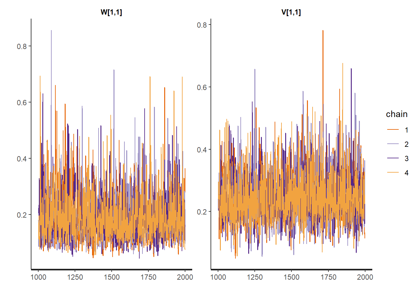
# パラメータのdensity plot
stan_dens(mcmc_result)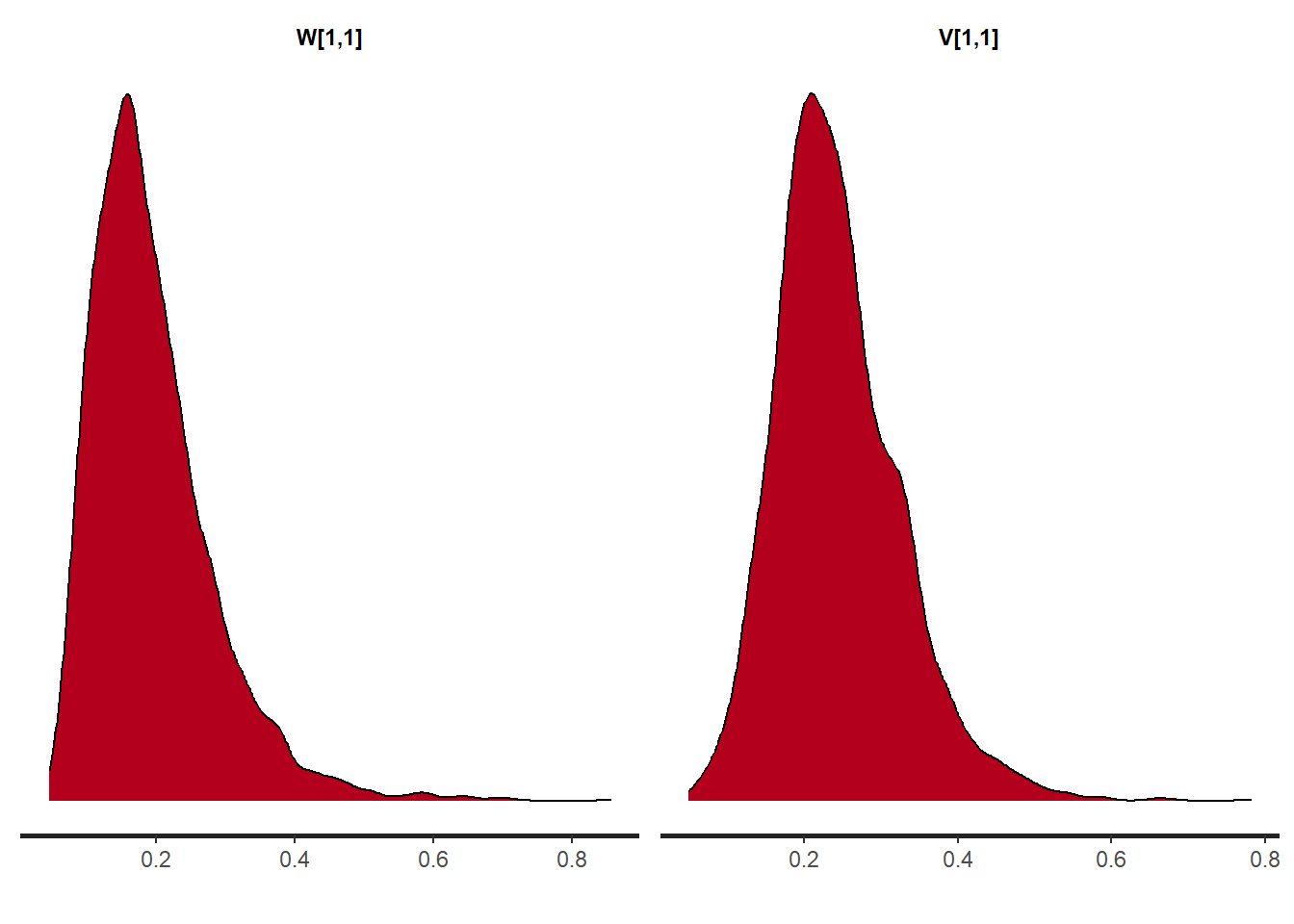
mcmc_sample <- rstan::extract(mcmc_result, permuted = T, pars = c("W", "V"))
str(mcmc_sample)
List of 2
$ W: num [1:4000, 1, 1] 0.1835 0.1388 0.158 0.0844 0.1851 ...
..- attr(*, "dimnames")=List of 3
.. ..$ iterations: NULL
.. ..$ : NULL
.. ..$ : NULL
$ V: num [1:4000, 1, 1] 0.301 0.162 0.277 0.26 0.214 ...
..- attr(*, "dimnames")=List of 3
.. ..$ iterations: NULL
.. ..$ : NULL
.. ..$ : NULLmcmc_sample$W %>%
class()
mcmc_sample$W[1:5, 1, 1][1] "array"
[1] 0.18348167 0.13878693 0.15802664 0.08437417 0.18508070mcmc_sample$V %>%
class()
mcmc_sample$V[1:5, 1, 1][1] "array"
[1] 0.3009825 0.1617626 0.2770155 0.2599409 0.2142439# FFBSで状態を再現。パッケージ dlm を利用します。
# R codeは 萩原淳一郎他(2018),『基礎からわかる時系列分析』,技術評論社,pp.198-199 より引用
# Forward filtering-Backward sampling (FFBS)
# https://www.jstage.jst.go.jp/article/pjsai/JSAI2020/0/JSAI2020_1Q5GS1103/_pdf
# dlmFilter {dlm} 『The functions applies Kalman filter to compute filtered values of the state vectors,
# together with their variance/covariance matrices. 』
# dlmBSample {dlm} 『The function simulates one draw from the posterior distribution of the state vectors.』
mod <- dlm::dlmModPoly(order = 1, dV = V[1, 1], dW = W[1, 1], m0 = m0, C0 = C0[1, 1])
# 試行1回目(it = 1)
mod$W[1, 1] <- mcmc_sample$W[1, 1, 1]
mod$V[1, 1] <- mcmc_sample$V[1, 1, 1]
modFilt <- dlm::dlmFilter(y = y, mod = mod)
# str(modFilt)
x_FFBS <- dlm::dlmBSample(modFilt = modFilt)
str(x_FFBS) num [1:51, 1] 9.84 9.2 9.55 9.42 9.38 ...it_seq <- seq_along(along.with = mcmc_sample$V[, 1, 1])
head(it_seq)
tail(it_seq)[1] 1 2 3 4 5 6
[1] 3995 3996 3997 3998 3999 4000x_FFBS <- sapply(it_seq, function(it) {
mod$W[1, 1] <- mcmc_sample$W[it, 1, 1]
mod$V[1, 1] <- mcmc_sample$V[it, 1, 1]
return(dlm::dlmBSample(modFilt = dlm::dlmFilter(y = y, mod = mod)))
})
dim(x_FFBS)[1] 51 4000library(ggplot2)
x_FFBS <- t(x_FFBS[-1, ])
s_FFBS <- colMeans(x_FFBS)
# dlmSmooth {dlm} 『The function apply Kalman smoother to compute smoothed values of the state vectors,
# together with their variance/covariance matrices.』
dlmSmoothed_obj <- dlm::dlmSmooth(y = y, mod = mod)
mu <- dlmSmoothed_obj$s %>%
dlm::dropFirst()
ggplot(mapping = aes(x = seq(N))) + geom_line(mapping = aes(y = y[1, ])) + geom_point(mapping = aes(y = y[1, ])) + geom_line(mapping = aes(y = s_FFBS, color = "FFBS")) + geom_line(mapping = aes(y = mu, color = "dlmSmooth")) + theme(legend.title = element_blank())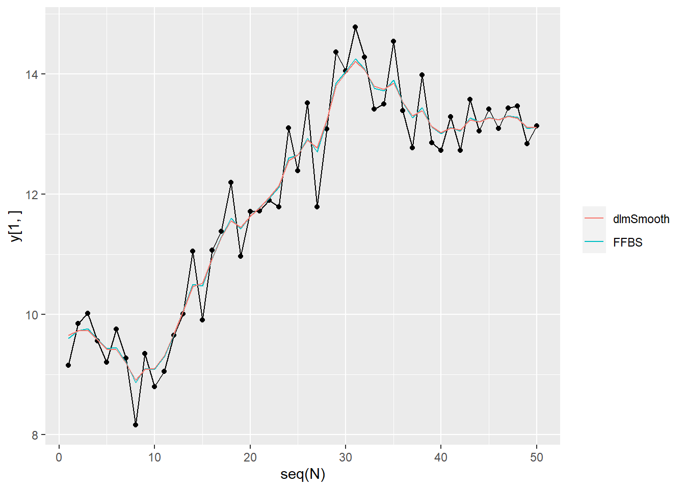
Sys.time()[1] "2024-03-12 13:40:59 JST"R.Version()$version.string[1] "R version 4.3.2 Patched (2023-12-27 r85754 ucrt)"quarto::quarto_version()[1] '1.4.542'packageVersion(pkg = "tidyverse")[1] '2.0.0'