library(rstan)
library(dplyr)
rstan_options(auto_write = TRUE)
options(mc.cores = parallel::detectCores())
packageVersion("rstan")
[1] '2.32.6'Rでデータサイエンス
library(rstan)
library(dplyr)
rstan_options(auto_write = TRUE)
options(mc.cores = parallel::detectCores())
packageVersion("rstan")[1] '2.32.6'# sample data
y <- m0 <- x0_gamma <- x_mu <- x_gamma <- vector()
# 整数
N <- 50
# ベクトル
m0 <- c(1, rep(0.5, 11)) # 事前分布の平均ベクトル
# 行列
C0 <- diag(x = 0.1, nrow = 12)
V <- matrix(0.1)
# 実数(下限=0)
W_mu <- 0.2
W_gamma <- 0.3
# 状態方程式 レベル成分の事前分布
x0_mu <- rnorm(n = 1, mean = m0[1], sd = sqrt(C0[1, 1]))
## レベル成分
x_mu[1] <- rnorm(n = 1, mean = x0_mu, sd = sqrt(W_mu))
for (t in 2:N) {
x_mu[t] <- rnorm(n = 1, mean = x_mu[t - 1], sd = sqrt(W_mu))
}
plot(x_mu, type = "o")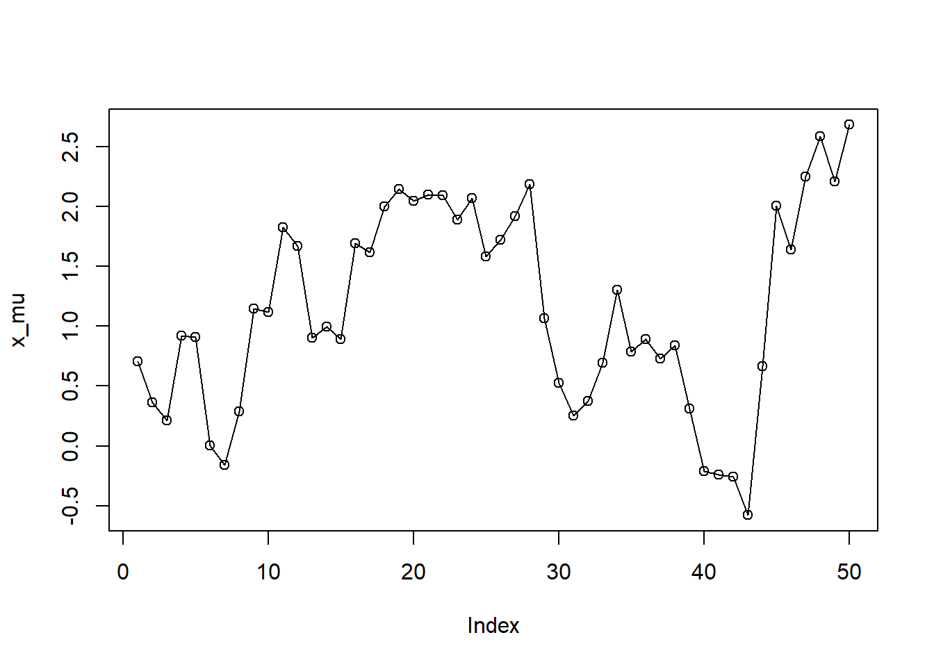
## 周期成分の事前分布
for (p in 1:11) {
    x0_gamma[p] <- rnorm(n = 1, mean = m0[p + 1], sd = sqrt(C0[p + 1, p + 1]))
}
plot(x0_gamma, type = "o")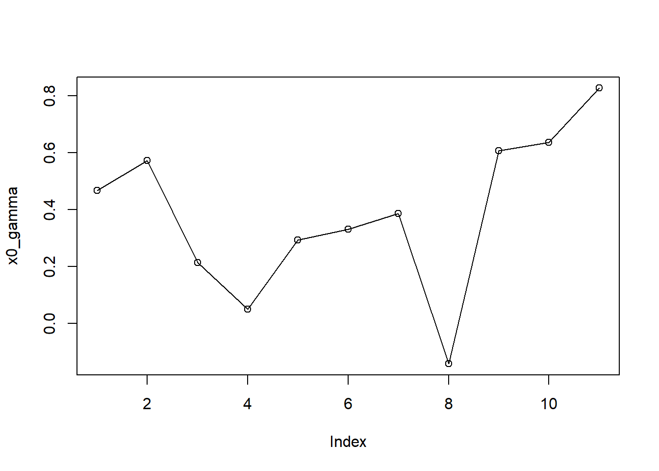
x_gamma[1] <- rnorm(n = 1, mean = -sum(x0_gamma), sd = sqrt(W_gamma))
for (t in 2:11) {
    x_gamma[t] <- rnorm(n = 1, mean = -sum(x0_gamma[t:11]) - sum(x_gamma[1:(t - 1)]), sd = sqrt(W_gamma))
}
plot(x_gamma, type = "o")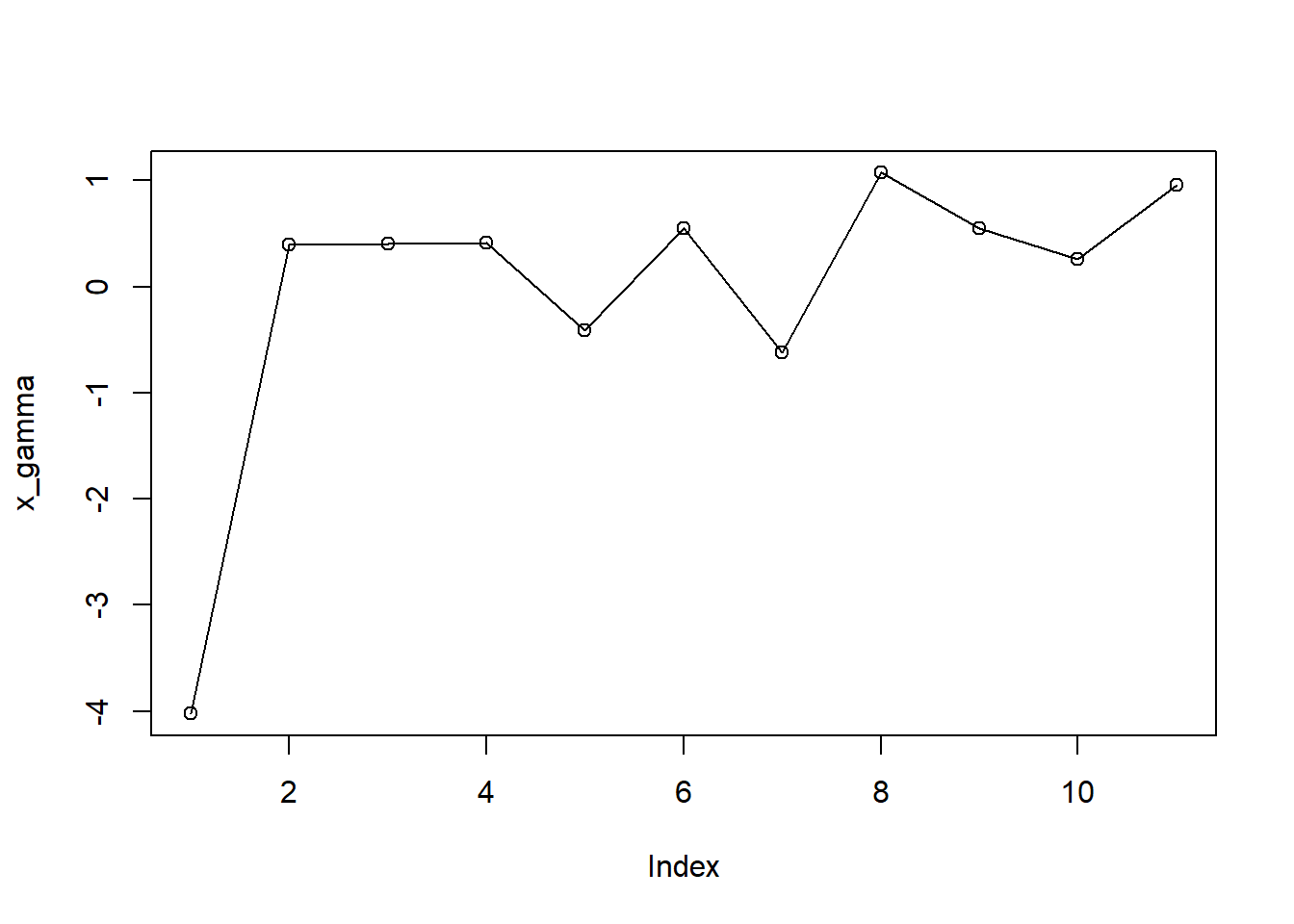
for (t in 12:N) {
    x_gamma[t] <- rnorm(n = 1, mean = -sum(x_gamma[(t - 11):(t - 1)]), sd = sqrt(W_gamma))
}
plot(x_gamma, type = "o")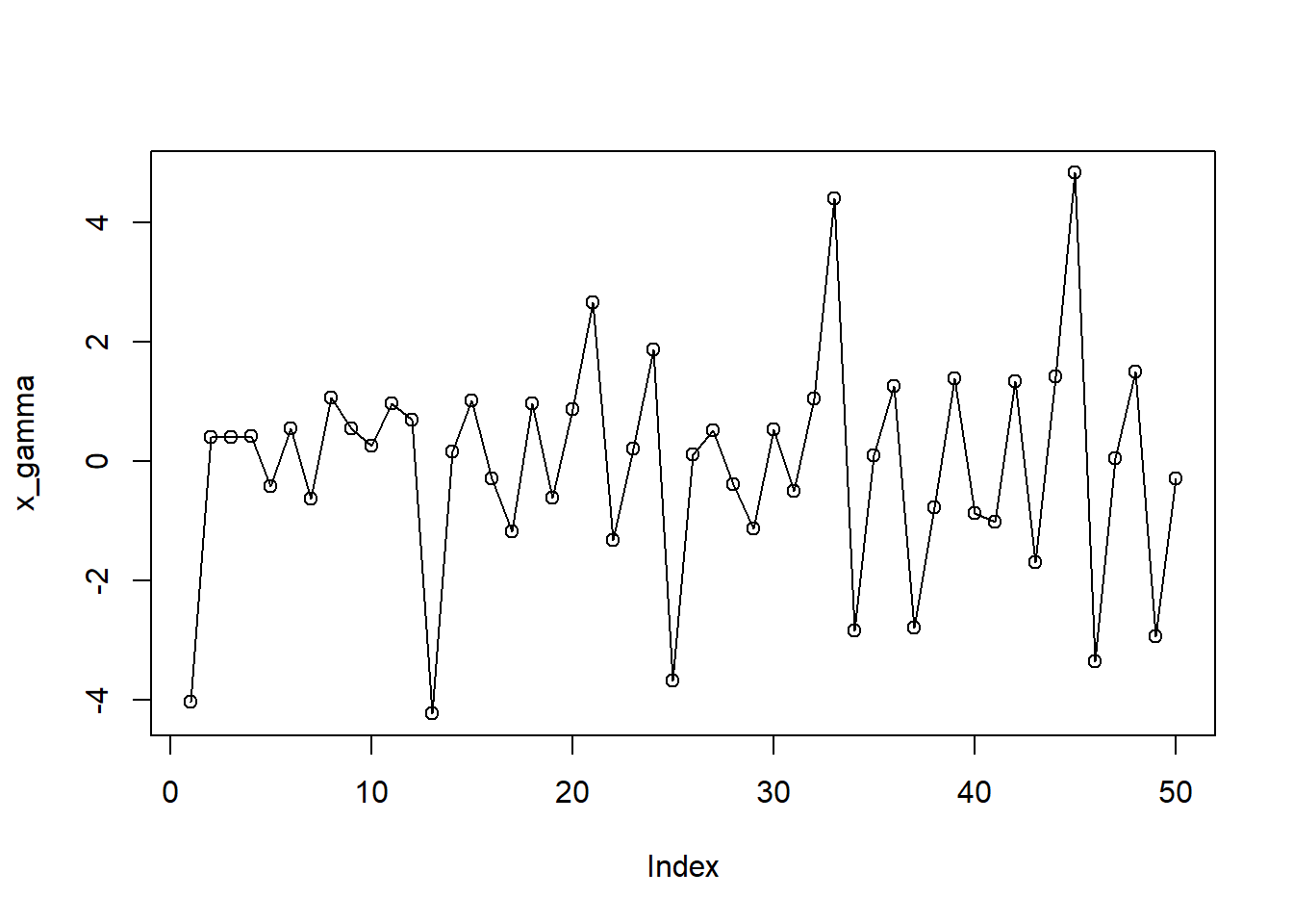
# 観測方程式
for (t in 1:N) {
    y[t] <- rnorm(n = 1, mean = x_mu[t] + x_gamma[t], sd = sqrt(V[1, 1]))
}
plot(y, type = "o")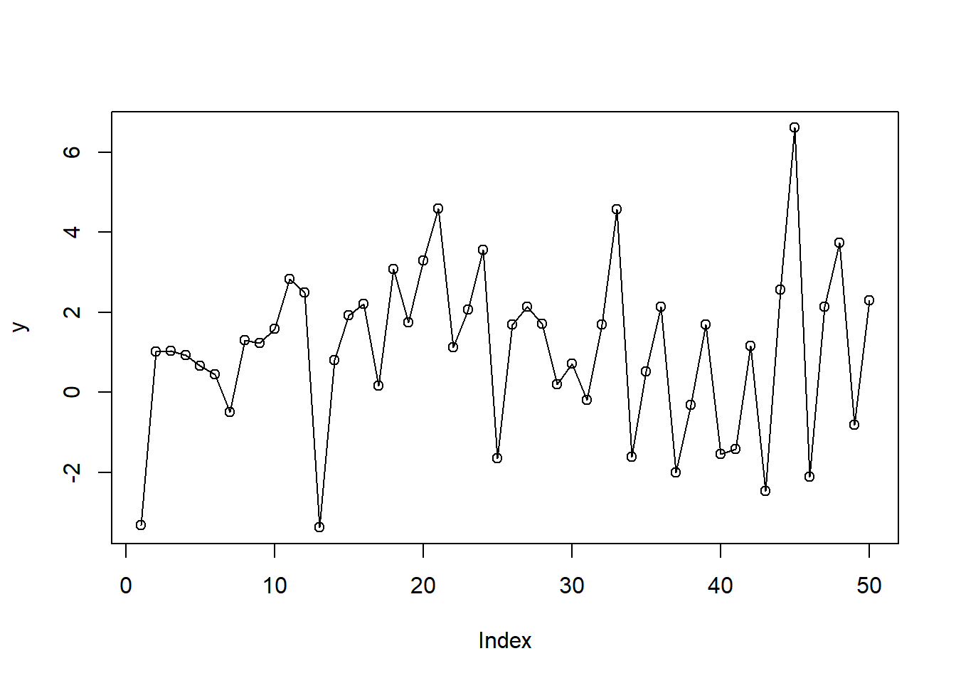
# stan code
model_code = '
data{
  int<lower=1> N; // 時系列データの要素数
  vector[N] y; // 観測値
  // 事前分布
  vector[12] m0; // 平均ベクトル
  cov_matrix[12] C0; // 分散,正定値対称行列 共分散行列 (p × p)行列
}

parameters{
  // 状態のレベル成分
  real x0_mu; // [0]
  vector[N] x_mu; // [1:N]

  // 状態の周期成分
  vector[11] x0_gamma; // [0]
  vector[N] x_gamma; // [1:N]

  // 状態雑音
  real<lower=0> W_mu; // レベル成分の分散
  real<lower=0> W_gamma; // 周期成分の分散
  // 観測雑音
  cov_matrix[1] V; // 共分散行列
}

// よってW_mu、W_gammaおよびVの事前分布は、指定しない場合のStanのデフォルトである、無情報事前分布となる。

model{
  // 観測方程式
  for(t in 1:N){
    y[t] ~ normal(x_mu[t] + x_gamma[t], sqrt(V[1,1]));
  }

  // 状態方程式
  //// レベル成分の事前分布
  x0_mu ~ normal(m0[1], sqrt(C0[1,1]));

  //// レベル成分
  x_mu[1] ~ normal(x0_mu, sqrt(W_mu));
  for(t in 2:N){
    x_mu[t] ~ normal(x_mu[t-1], sqrt(W_mu));
  }

  //// 周期成分の事前分布
  for(p in 1:11){
    x0_gamma[p] ~ normal(m0[p+1], sqrt(C0[(p+1), (p+1)]));
  }

  //// 周期成分
  x_gamma[1] ~ normal(-sum(x0_gamma[1:11]), sqrt(W_gamma));
  for(t in 2:11){
    x_gamma[t] ~ normal(-sum(x0_gamma[t:11]) - sum(x_gamma[1:(t-1)]), sqrt(W_gamma));
  }
  for(t in 12:N){
    x_gamma[t] ~ normal(-sum(x_gamma[(t-11):(t-1)]), sqrt(W_gamma));
  }
}
'data_list <- list(N = N, y = y, m0 = m0, C0 = C0)
mcmc_result <- stan(model_code = model_code, data = data_list, refresh = 0)# パラメータの平均、標準偏差、信用区間、R hat の確認
print(mcmc_result, pars = c("W_mu", "W_gamma", "V[1,1]"))Inference for Stan model: anon_model.
4 chains, each with iter=2000; warmup=1000; thin=1;
post-warmup draws per chain=1000, total post-warmup draws=4000.
mean se_mean sd 2.5% 25% 50% 75% 97.5% n_eff Rhat
W_mu 0.27 0.01 0.16 0.07 0.16 0.23 0.34 0.67 560 1.01
W_gamma 0.45 0.00 0.17 0.21 0.34 0.42 0.53 0.87 1260 1.00
V[1,1] 0.20 0.01 0.19 0.01 0.06 0.15 0.28 0.69 232 1.01
Samples were drawn using NUTS(diag_e) at Thu Mar 14 08:38:37 2024.
For each parameter, n_eff is a crude measure of effective sample size,
and Rhat is the potential scale reduction factor on split chains (at
convergence, Rhat=1).# パラメータの平均、標準偏差、信用区間、R hat の確認
print(mcmc_result, pars = "x0_mu")Inference for Stan model: anon_model.
4 chains, each with iter=2000; warmup=1000; thin=1;
post-warmup draws per chain=1000, total post-warmup draws=4000.
mean se_mean sd 2.5% 25% 50% 75% 97.5% n_eff Rhat
x0_mu 0.97 0 0.28 0.43 0.78 0.97 1.17 1.51 4980 1
Samples were drawn using NUTS(diag_e) at Thu Mar 14 08:38:37 2024.
For each parameter, n_eff is a crude measure of effective sample size,
and Rhat is the potential scale reduction factor on split chains (at
convergence, Rhat=1).# パラメータの平均、標準偏差、信用区間、R hat の確認
print(mcmc_result, pars = "x0_gamma")Inference for Stan model: anon_model.
4 chains, each with iter=2000; warmup=1000; thin=1;
post-warmup draws per chain=1000, total post-warmup draws=4000.
mean se_mean sd 2.5% 25% 50% 75% 97.5% n_eff Rhat
x0_gamma[1] 0.42 0 0.31 -0.19 0.21 0.42 0.62 1.04 6275 1
x0_gamma[2] 0.39 0 0.29 -0.17 0.19 0.39 0.59 0.96 5441 1
x0_gamma[3] 0.33 0 0.29 -0.24 0.13 0.34 0.53 0.92 5642 1
x0_gamma[4] 0.29 0 0.28 -0.26 0.11 0.29 0.47 0.84 4839 1
x0_gamma[5] 0.30 0 0.29 -0.27 0.10 0.30 0.50 0.86 4329 1
x0_gamma[6] 0.29 0 0.29 -0.29 0.09 0.30 0.49 0.85 4093 1
x0_gamma[7] 0.46 0 0.29 -0.11 0.26 0.46 0.66 1.03 4441 1
x0_gamma[8] 0.50 0 0.30 -0.09 0.30 0.50 0.70 1.10 4705 1
x0_gamma[9] 0.48 0 0.30 -0.10 0.27 0.47 0.69 1.03 4042 1
x0_gamma[10] 0.56 0 0.30 -0.01 0.35 0.56 0.76 1.13 3822 1
x0_gamma[11] 0.57 0 0.31 -0.02 0.37 0.57 0.77 1.18 5475 1
Samples were drawn using NUTS(diag_e) at Thu Mar 14 08:38:37 2024.
For each parameter, n_eff is a crude measure of effective sample size,
and Rhat is the potential scale reduction factor on split chains (at
convergence, Rhat=1).# パラメータの平均、標準偏差、信用区間、R hat の確認
print(mcmc_result, pars = "x_mu")Inference for Stan model: anon_model.
4 chains, each with iter=2000; warmup=1000; thin=1;
post-warmup draws per chain=1000, total post-warmup draws=4000.
mean se_mean sd 2.5% 25% 50% 75% 97.5% n_eff Rhat
x_mu[1] 0.91 0.01 0.37 0.19 0.67 0.91 1.15 1.66 3060 1
x_mu[2] 0.80 0.01 0.37 0.08 0.56 0.80 1.03 1.52 3268 1
x_mu[3] 0.65 0.01 0.36 -0.10 0.42 0.65 0.88 1.33 3594 1
x_mu[4] 0.56 0.01 0.35 -0.15 0.34 0.57 0.80 1.25 3332 1
x_mu[5] 0.51 0.01 0.36 -0.23 0.27 0.51 0.74 1.22 4000 1
x_mu[6] 0.24 0.01 0.39 -0.53 -0.02 0.25 0.49 0.98 1573 1
x_mu[7] 0.18 0.01 0.40 -0.64 -0.07 0.18 0.44 0.97 1642 1
x_mu[8] 0.39 0.01 0.39 -0.38 0.14 0.39 0.63 1.13 2245 1
x_mu[9] 0.69 0.01 0.37 -0.05 0.45 0.70 0.94 1.39 3600 1
x_mu[10] 1.30 0.01 0.40 0.58 1.03 1.28 1.56 2.13 1682 1
x_mu[11] 1.63 0.01 0.43 0.82 1.33 1.60 1.91 2.51 1187 1
x_mu[12] 1.42 0.01 0.38 0.69 1.17 1.42 1.66 2.21 2211 1
x_mu[13] 1.12 0.01 0.38 0.38 0.88 1.13 1.37 1.87 2783 1
x_mu[14] 1.09 0.01 0.38 0.32 0.86 1.09 1.33 1.82 2298 1
x_mu[15] 1.28 0.01 0.37 0.54 1.03 1.28 1.52 1.99 3106 1
x_mu[16] 1.48 0.01 0.37 0.74 1.24 1.48 1.72 2.20 3419 1
x_mu[17] 1.59 0.01 0.38 0.78 1.35 1.61 1.86 2.31 1769 1
x_mu[18] 2.06 0.01 0.38 1.26 1.82 2.07 2.30 2.78 2489 1
x_mu[19] 2.26 0.01 0.38 1.49 2.03 2.27 2.51 3.01 2418 1
x_mu[20] 2.29 0.01 0.38 1.52 2.04 2.29 2.54 3.06 2184 1
x_mu[21] 2.24 0.01 0.37 1.54 2.00 2.23 2.47 2.98 2523 1
x_mu[22] 2.14 0.01 0.37 1.44 1.90 2.12 2.38 2.88 2503 1
x_mu[23] 2.03 0.01 0.37 1.33 1.77 2.02 2.27 2.77 2967 1
x_mu[24] 2.04 0.01 0.39 1.32 1.78 2.02 2.28 2.85 2189 1
x_mu[25] 1.94 0.01 0.40 1.21 1.66 1.92 2.19 2.78 2178 1
x_mu[26] 1.77 0.01 0.39 1.01 1.52 1.75 2.01 2.58 2578 1
x_mu[27] 1.49 0.01 0.39 0.72 1.25 1.50 1.75 2.24 2877 1
x_mu[28] 1.35 0.01 0.38 0.58 1.11 1.36 1.60 2.07 2990 1
x_mu[29] 1.04 0.01 0.39 0.22 0.79 1.06 1.30 1.78 1846 1
x_mu[30] 0.69 0.01 0.43 -0.25 0.44 0.72 0.98 1.44 1165 1
x_mu[31] 0.77 0.01 0.38 -0.01 0.52 0.77 1.02 1.51 2465 1
x_mu[32] 0.72 0.01 0.38 -0.04 0.47 0.72 0.97 1.50 2813 1
x_mu[33] 0.73 0.01 0.39 0.00 0.47 0.72 0.99 1.53 2595 1
x_mu[34] 0.65 0.01 0.37 -0.05 0.40 0.63 0.88 1.40 2894 1
x_mu[35] 0.58 0.01 0.38 -0.15 0.34 0.58 0.83 1.31 2903 1
x_mu[36] 0.64 0.01 0.39 -0.10 0.38 0.63 0.89 1.45 1691 1
x_mu[37] 0.64 0.01 0.42 -0.14 0.35 0.62 0.90 1.54 1306 1
x_mu[38] 0.32 0.01 0.41 -0.46 0.05 0.31 0.57 1.16 2018 1
x_mu[39] 0.06 0.01 0.40 -0.75 -0.20 0.06 0.32 0.85 2769 1
x_mu[40] -0.33 0.01 0.47 -1.31 -0.63 -0.31 -0.01 0.55 1142 1
x_mu[41] -0.29 0.01 0.47 -1.24 -0.59 -0.28 0.02 0.58 1016 1
x_mu[42] -0.02 0.01 0.43 -0.92 -0.29 0.00 0.26 0.78 1361 1
x_mu[43] 0.25 0.01 0.44 -0.67 -0.01 0.26 0.53 1.06 1371 1
x_mu[44] 0.90 0.01 0.40 0.13 0.64 0.89 1.15 1.75 3074 1
x_mu[45] 1.37 0.01 0.42 0.61 1.09 1.34 1.64 2.24 1809 1
x_mu[46] 1.48 0.01 0.40 0.72 1.21 1.46 1.75 2.26 3132 1
x_mu[47] 1.79 0.01 0.41 1.00 1.51 1.77 2.04 2.61 2389 1
x_mu[48] 2.05 0.01 0.43 1.24 1.75 2.03 2.34 2.91 1549 1
x_mu[49] 2.23 0.01 0.49 1.31 1.89 2.21 2.55 3.24 1342 1
x_mu[50] 2.35 0.02 0.61 1.24 1.94 2.33 2.74 3.63 1343 1
Samples were drawn using NUTS(diag_e) at Thu Mar 14 08:38:37 2024.
For each parameter, n_eff is a crude measure of effective sample size,
and Rhat is the potential scale reduction factor on split chains (at
convergence, Rhat=1).# パラメータの平均、標準偏差、信用区間、R hat の確認
print(mcmc_result, pars = "x_gamma")Inference for Stan model: anon_model.
4 chains, each with iter=2000; warmup=1000; thin=1;
post-warmup draws per chain=1000, total post-warmup draws=4000.
mean se_mean sd 2.5% 25% 50% 75% 97.5% n_eff Rhat
x_gamma[1] -4.25 0.01 0.46 -5.16 -4.55 -4.25 -3.94 -3.33 2977 1
x_gamma[2] 0.20 0.01 0.40 -0.62 -0.06 0.21 0.47 0.98 3968 1
x_gamma[3] 0.43 0.01 0.40 -0.34 0.16 0.43 0.70 1.22 4085 1
x_gamma[4] 0.38 0.01 0.40 -0.42 0.12 0.38 0.63 1.19 3667 1
x_gamma[5] 0.05 0.01 0.41 -0.79 -0.20 0.05 0.32 0.83 3600 1
x_gamma[6] 0.35 0.01 0.41 -0.44 0.07 0.34 0.62 1.19 2213 1
x_gamma[7] -0.45 0.01 0.41 -1.22 -0.73 -0.46 -0.18 0.39 2769 1
x_gamma[8] 0.99 0.01 0.42 0.14 0.73 1.00 1.25 1.81 4227 1
x_gamma[9] 0.75 0.01 0.43 -0.05 0.45 0.73 1.03 1.66 2055 1
x_gamma[10] 0.07 0.01 0.44 -0.87 -0.21 0.09 0.37 0.88 1907 1
x_gamma[11] 0.86 0.01 0.46 -0.06 0.55 0.87 1.17 1.72 1066 1
x_gamma[12] 1.01 0.01 0.42 0.18 0.74 1.02 1.28 1.84 2837 1
x_gamma[13] -4.31 0.01 0.43 -5.14 -4.60 -4.33 -4.03 -3.44 2330 1
x_gamma[14] -0.12 0.01 0.42 -0.96 -0.39 -0.12 0.16 0.71 2732 1
x_gamma[15] 0.69 0.01 0.42 -0.13 0.41 0.68 0.96 1.54 3841 1
x_gamma[16] 0.68 0.01 0.43 -0.17 0.41 0.69 0.97 1.49 3030 1
x_gamma[17] -1.19 0.01 0.48 -2.05 -1.53 -1.22 -0.89 -0.19 1062 1
x_gamma[18] 0.85 0.01 0.43 0.00 0.57 0.84 1.14 1.71 3055 1
x_gamma[19] -0.66 0.01 0.42 -1.54 -0.94 -0.66 -0.39 0.18 3914 1
x_gamma[20] 0.93 0.01 0.42 0.11 0.66 0.93 1.21 1.77 3161 1
x_gamma[21] 2.30 0.01 0.43 1.44 2.02 2.31 2.58 3.12 3516 1
x_gamma[22] -1.03 0.01 0.42 -1.88 -1.30 -1.03 -0.75 -0.19 3644 1
x_gamma[23] 0.13 0.01 0.43 -0.72 -0.16 0.13 0.41 0.99 2884 1
x_gamma[24] 1.45 0.01 0.45 0.50 1.15 1.47 1.75 2.29 1867 1
x_gamma[25] -3.64 0.01 0.45 -4.53 -3.93 -3.63 -3.34 -2.78 2570 1
x_gamma[26] -0.14 0.01 0.43 -1.02 -0.40 -0.12 0.13 0.69 2528 1
x_gamma[27] 0.71 0.01 0.44 -0.10 0.42 0.70 1.00 1.64 2443 1
x_gamma[28] 0.24 0.01 0.43 -0.60 -0.05 0.24 0.53 1.07 3139 1
x_gamma[29] -0.82 0.01 0.46 -1.70 -1.12 -0.83 -0.53 0.12 1915 1
x_gamma[30] 0.28 0.02 0.49 -0.59 -0.07 0.25 0.58 1.36 878 1
x_gamma[31] -1.01 0.01 0.43 -1.86 -1.29 -1.00 -0.72 -0.16 2851 1
x_gamma[32] 1.01 0.01 0.44 0.15 0.71 1.01 1.30 1.86 3349 1
x_gamma[33] 3.78 0.01 0.46 2.81 3.49 3.82 4.09 4.63 1652 1
x_gamma[34] -2.22 0.01 0.43 -3.07 -2.50 -2.22 -1.94 -1.38 3092 1
x_gamma[35] 0.01 0.01 0.44 -0.82 -0.28 0.00 0.31 0.90 2795 1
x_gamma[36] 1.45 0.01 0.45 0.55 1.15 1.44 1.74 2.33 2040 1
x_gamma[37] -2.84 0.02 0.50 -3.93 -3.15 -2.82 -2.50 -1.94 1033 1
x_gamma[38] -0.57 0.01 0.47 -1.53 -0.88 -0.57 -0.28 0.35 2268 1
x_gamma[39] 1.58 0.01 0.49 0.60 1.27 1.59 1.90 2.52 2914 1
x_gamma[40] -0.91 0.02 0.53 -1.88 -1.28 -0.93 -0.56 0.22 1128 1
x_gamma[41] -0.93 0.01 0.51 -1.89 -1.28 -0.95 -0.60 0.10 1446 1
x_gamma[42] 1.20 0.01 0.49 0.22 0.89 1.19 1.52 2.21 2100 1
x_gamma[43] -2.43 0.02 0.53 -3.37 -2.79 -2.47 -2.11 -1.27 1113 1
x_gamma[44] 1.54 0.01 0.50 0.47 1.22 1.56 1.88 2.48 2122 1
x_gamma[45] 4.97 0.02 0.55 3.75 4.62 5.02 5.35 5.93 1014 1
x_gamma[46] -3.43 0.01 0.51 -4.38 -3.76 -3.46 -3.11 -2.36 2051 1
x_gamma[47] 0.31 0.01 0.45 -0.61 0.02 0.31 0.61 1.19 2857 1
x_gamma[48] 1.61 0.01 0.50 0.56 1.30 1.62 1.94 2.56 2180 1
x_gamma[49] -3.10 0.01 0.53 -4.17 -3.44 -3.09 -2.73 -2.09 1670 1
x_gamma[50] -0.16 0.02 0.63 -1.44 -0.57 -0.14 0.26 1.07 1485 1
Samples were drawn using NUTS(diag_e) at Thu Mar 14 08:38:37 2024.
For each parameter, n_eff is a crude measure of effective sample size,
and Rhat is the potential scale reduction factor on split chains (at
convergence, Rhat=1).# トレースプロットで収束度合いの確認
traceplot(object = mcmc_result, pars = c("W_mu", "W_gamma", "V[1,1]"))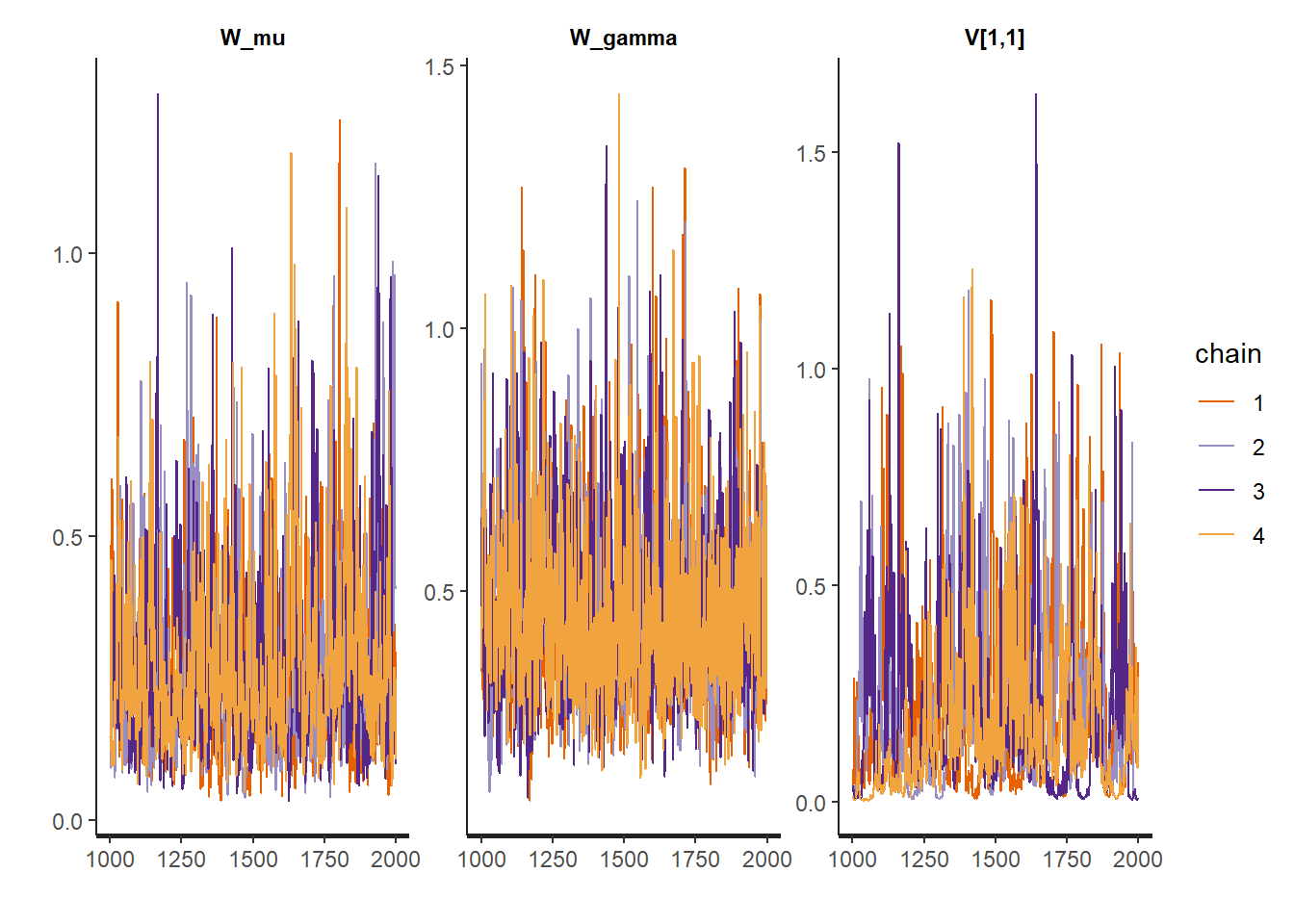
stan_dens(object = mcmc_result, pars = c("W_mu", "W_gamma", "V[1,1]"))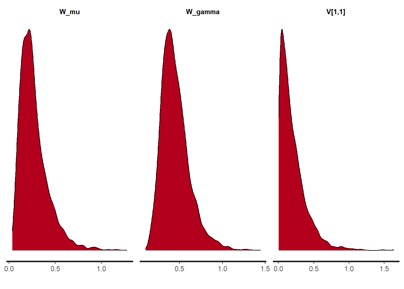
mcmc_sample <- rstan::extract(mcmc_result, permuted = T)
mu <- mcmc_sample$x_mu + mcmc_sample$x_gamma
dim(mu)
[1] 4000 50sample_df <- data.frame(x = seq(N), y = y, muM = apply(mu, 2, mean), muL = apply(mu, 2, quantile, 0.025), muU = apply(mu, 2, quantile, 0.925))
sample_df %>%
ggplot(mapping = aes(x = x, y = y)) + geom_point() + geom_smooth(mapping = aes(ymin = muL, ymax = muU, y = muM), color = "blue", stat = "identity")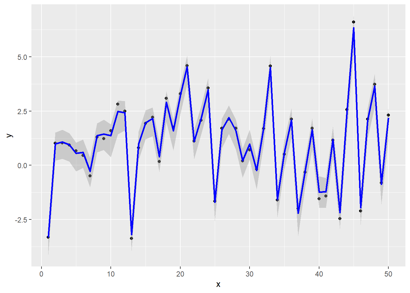
Sys.time()[1] "2024-03-14 08:38:44 JST"R.Version()$version.string[1] "R version 4.3.2 Patched (2023-12-27 r85754 ucrt)"quarto::quarto_version()[1] '1.4.542'packageVersion(pkg = "tidyverse")[1] '2.0.0'