Rで統計的仮説検定:アンサリ･ブラッドリー検定

Rでデータサイエンス

アンサリ･ブラッドリー検定

中央値の等しい2つの群の分散(scale)同一性の検定
ノンパラメトリック検定(正規分布に従わない群に利用できる)
帰無仮説:2つの群の分散(scale)は等しい

サンプル

# 関数
library(dplyr)
library(ggplot2)
seed <- 20230430
location_x <- location_y <- 50
fun_sim <- function(n_x, n_y, location_x, location_y, scale_x, scale_y) {
    x <- rlogis(n = n_x, location = location_x, scale = scale_x)
    y <- rlogis(n = n_y, location = location_y, scale = scale_y)
    value <- c(x, y)
    key <- c(rep("x", n_x), rep("y", n_y))
    df <- data.frame(key, value)
    g <- ggplot(data = df, mapping = aes(x = value, fill = key)) + geom_histogram(col = "white", position = "identity", alpha = 0.7) + theme_minimal() + theme(legend.title = element_blank())
    result_ansari <- ansari.test(x, y, alternative = "two.sided")
    return(list(g = g, result_ansari = result_ansari, result_median = list(x = median(x), y = median(y))))
}
# 以降有意水準は5%とする。

set.seed(seed = seed)
# サンプルサイズは同一
n_x <- 100
n_y <- 100
# 分散は同一
scale_x <- 3
scale_y <- 3
fun_sim(n_x = n_x, n_y = n_y, location_x = location_x, location_y = location_y, scale_x = scale_x, scale_y = scale_y)
# 帰無仮説は棄却されない。

$g

$result_ansari

    Ansari-Bradley test

data:  x and y
AB = 5047, p-value = 0.9883
alternative hypothesis: true ratio of scales is not equal to 1


$result_median
$result_median$x
[1] 49.07661

$result_median$y
[1] 51.37151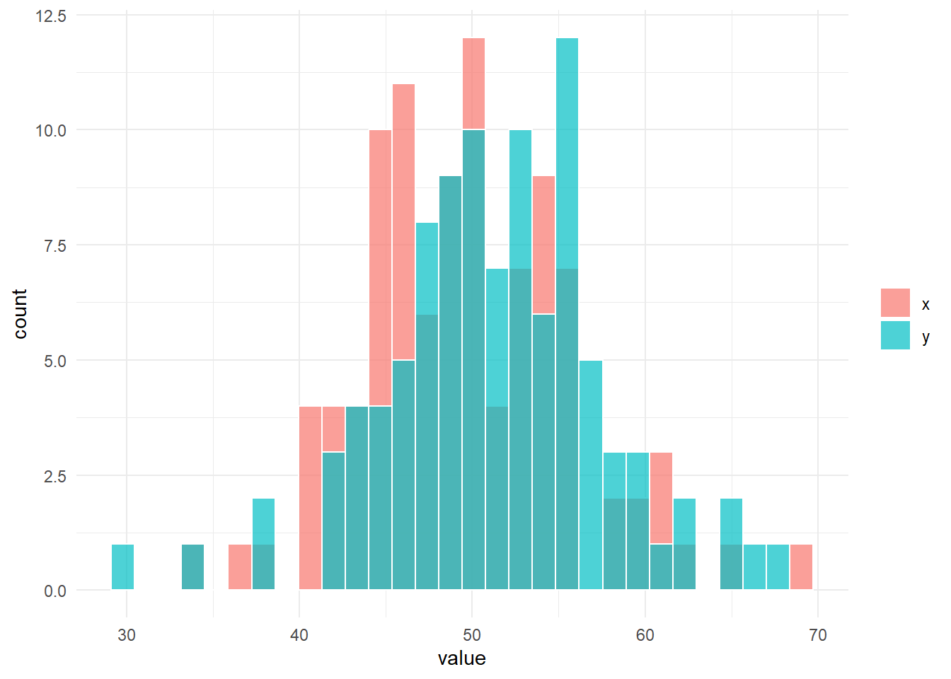

set.seed(seed = seed)
# サンプルサイズは同一
n_x <- 100
n_y <- 100
# 分散は異なる
scale_x <- 3
scale_y <- 5
fun_sim(n_x = n_x, n_y = n_y, location_x = location_x, location_y = location_y, scale_x = scale_x, scale_y = scale_y)
# 帰無仮説は棄却される。

$g

$result_ansari

    Ansari-Bradley test

data:  x and y
AB = 5749, p-value = 0.0006355
alternative hypothesis: true ratio of scales is not equal to 1


$result_median
$result_median$x
[1] 49.07661

$result_median$y
[1] 52.28586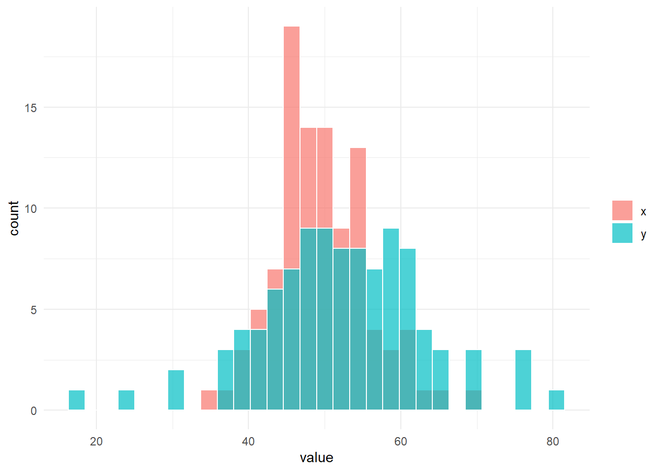

set.seed(seed = seed)
# サンプルサイズは異なる
n_x <- 100
n_y <- 200
# 分散は同一
scale_x <- 3
scale_y <- 3
fun_sim(n_x = n_x, n_y = n_y, location_x = location_x, location_y = location_y, scale_x = scale_x, scale_y = scale_y)
# 帰無仮説は棄却されない。

$g

$result_ansari

    Ansari-Bradley test

data:  x and y
AB = 7194, p-value = 0.3148
alternative hypothesis: true ratio of scales is not equal to 1


$result_median
$result_median$x
[1] 49.07661

$result_median$y
[1] 50.73988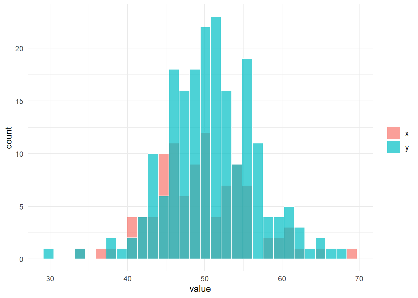

set.seed(seed = seed)
# サンプルサイズは異なる
n_x <- 100
n_y <- 200
# 分散は異なる
scale_x <- 3
scale_y <- 5
fun_sim(n_x = n_x, n_y = n_y, location_x = location_x, location_y = location_y, scale_x = scale_x, scale_y = scale_y)
# 帰無仮説は棄却される。

$g

$result_ansari

    Ansari-Bradley test

data:  x and y
AB = 8639, p-value = 0.002104
alternative hypothesis: true ratio of scales is not equal to 1


$result_median
$result_median$x
[1] 49.07661

$result_median$y
[1] 51.23313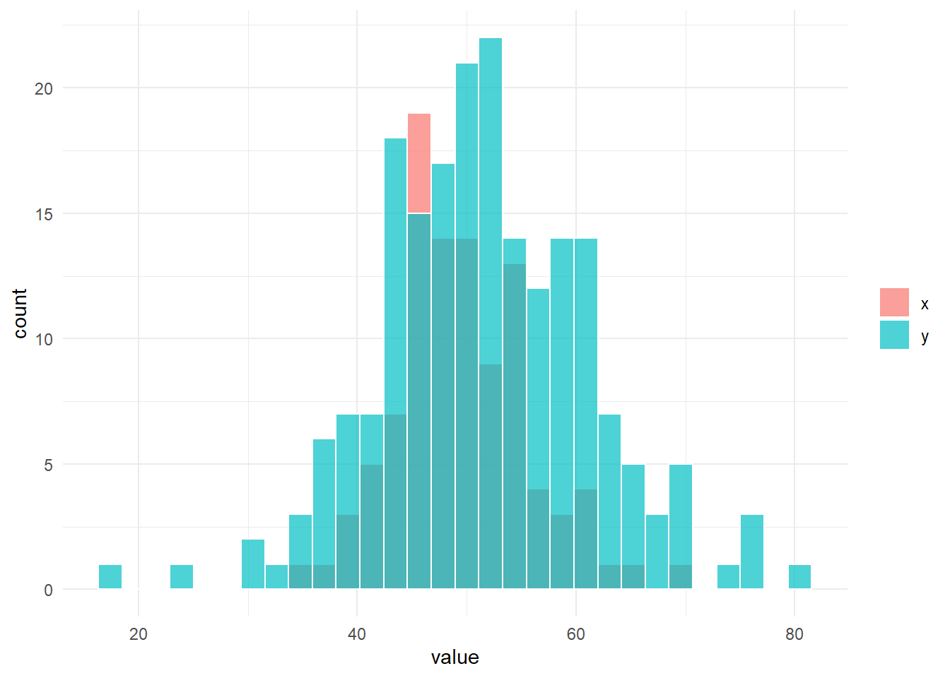

シミュレーション

set.seed(seed = seed)
iter <- 1000
result_ansari_p <- vector()
# サンプルサイズは同一
n_x <- 100
n_y <- 100
# 分散は同一
scale_x <- 3
scale_y <- 3
for (iii in seq(iter)) {
    result <- fun_sim(n_x = n_x, n_y = n_y, location_x = location_x, location_y = location_y, scale_x = scale_x, scale_y = scale_y)
    result_ansari_p[iii] <- result$result_ansari$p.value
}
sum(result_ansari_p < 0.05)/iter

[1] 0.053

set.seed(seed = seed)
iter <- 1000
result_ansari_p <- vector()
# サンプルサイズは同一
n_x <- 100
n_y <- 100
# 分散は異なる
scale_x <- 3
scale_y <- 5
for (iii in seq(iter)) {
    result <- fun_sim(n_x = n_x, n_y = n_y, location_x = location_x, location_y = location_y, scale_x = scale_x, scale_y = scale_y)
    result_ansari_p[iii] <- result$result_ansari$p.value
}
1 - sum(result_ansari_p < 0.05)/iter

[1] 0.061

set.seed(seed = seed)
iter <- 1000
result_ansari_p <- vector()
# サンプルサイズは異なる
n_x <- 100
n_y <- 200
# 分散は同一
scale_x <- 3
scale_y <- 3
for (iii in seq(iter)) {
    result <- fun_sim(n_x = n_x, n_y = n_y, location_x = location_x, location_y = location_y, scale_x = scale_x, scale_y = scale_y)
    result_ansari_p[iii] <- result$result_ansari$p.value
}
sum(result_ansari_p < 0.05)/iter

[1] 0.056

set.seed(seed = seed)
iter <- 1000
result_ansari_p <- vector()
# サンプルサイズは異なる
n_x <- 100
n_y <- 200
# 分散は異なる
scale_x <- 3
scale_y <- 5
for (iii in seq(iter)) {
    result <- fun_sim(n_x = n_x, n_y = n_y, location_x = location_x, location_y = location_y, scale_x = scale_x, scale_y = scale_y)
    result_ansari_p[iii] <- result$result_ansari$p.value
}
1 - sum(result_ansari_p < 0.05)/iter

[1] 0.015

コード

# 関数コード
methods("ansari.test")

[1] ansari.test.default* ansari.test.formula*
see '?methods' for accessing help and source code

getS3method(f = "ansari.test", class = "default")

function (x, y, alternative = c("two.sided", "less", "greater"), 
    exact = NULL, conf.int = FALSE, conf.level = 0.95, ...) 
{
    alternative <- match.arg(alternative)
    if (conf.int) {
        if (!((length(conf.level) == 1L) && is.finite(conf.level) && 
            (conf.level > 0) && (conf.level < 1))) 
            stop("'conf.level' must be a single number between 0 and 1")
    }
    DNAME <- paste(deparse1(substitute(x)), "and", deparse1(substitute(y)))
    x <- x[complete.cases(x)]
    y <- y[complete.cases(y)]
    m <- as.integer(length(x))
    if (is.na(m) || m < 1L) 
        stop("not enough 'x' observations")
    n <- as.integer(length(y))
    if (is.na(n) || n < 1L) 
        stop("not enough 'y' observations")
    N <- m + n
    r <- rank(c(x, y))
    STATISTIC <- sum(pmin(r, N - r + 1)[seq_along(x)])
    TIES <- (length(r) != length(unique(r)))
    if (is.null(exact)) 
        exact <- ((m < 50L) && (n < 50L))
    if (exact && !TIES) {
        pansari <- function(q, m, n) .Call(C_pAnsari, q, m, n)
        PVAL <- switch(alternative, two.sided = {
            if (STATISTIC > ((m + 1)^2%/%4 + ((m * n)%/%2)/2)) p <- 1 - 
                pansari(STATISTIC - 1, m, n) else p <- pansari(STATISTIC, 
                m, n)
            min(2 * p, 1)
        }, less = 1 - pansari(STATISTIC - 1, m, n), greater = pansari(STATISTIC, 
            m, n))
        if (conf.int) {
            qansari <- function(p, m, n) .Call(C_qAnsari, p, 
                m, n)
            alpha <- 1 - conf.level
            x <- sort(x)
            y <- sort(y)
            ab <- function(sig) {
                rab <- rank(c(x/sig, y))
                sum(pmin(rab, N - rab + 1)[seq_along(x)])
            }
            ratio <- outer(x, y, `/`)
            aratio <- ratio[ratio >= 0]
            sigma <- sort(aratio)
            cci <- function(alpha) {
                u <- absigma - qansari(alpha/2, m, n)
                l <- absigma - qansari(1 - alpha/2, m, n)
                if (length(u[u >= 0]) == 0L || length(l[l > 0]) == 
                  0L) {
                  warning("samples differ in location: cannot compute confidence set, returning NA")
                  return(c(NA, NA))
                }
                u[u < 0] <- NA
                uci <- min(sigma[which(u == min(u, na.rm = TRUE))])
                l[l <= 0] <- NA
                lci <- max(sigma[which(l == min(l, na.rm = TRUE))])
                if (uci > lci) {
                  l <- absigma - qansari(alpha/2, m, n)
                  u <- absigma - qansari(1 - alpha/2, m, n)
                  u[u < 0] <- NA
                  uci <- min(sigma[which(u == min(u, na.rm = TRUE))])
                  l[l <= 0] <- NA
                  lci <- max(sigma[which(l == min(l, na.rm = TRUE))])
                }
                c(uci, lci)
            }
            cint <- if (length(sigma) < 1L) {
                warning("cannot compute confidence set, returning NA")
                c(NA, NA)
            }
            else {
                absigma <- sapply(sigma + c(diff(sigma)/2, sigma[length(sigma)] * 
                  1.01), ab)
                switch(alternative, two.sided = cci(alpha), greater = c(cci(alpha * 
                  2)[1L], Inf), less = c(0, cci(alpha * 2)[2L]))
            }
            attr(cint, "conf.level") <- conf.level
            u <- absigma - qansari(0.5, m, n)
            sgr <- if (length(sgr <- sigma[u <= 0]) == 0L) 
                NA
            else max(sgr)
            sle <- if (length(sle <- sigma[u > 0]) == 0L) 
                NA
            else min(sle)
            ESTIMATE <- mean(c(sle, sgr))
        }
    }
    else {
        EVEN <- ((N%%2L) == 0L)
        normalize <- function(s, r, TIES, m = length(x), n = length(y)) {
            z <- if (EVEN) 
                s - m * (N + 2)/4
            else s - m * (N + 1)^2/(4 * N)
            if (!TIES) {
                SIGMA <- if (EVEN) 
                  sqrt((m * n * (N + 2) * (N - 2))/(48 * (N - 
                    1)))
                else sqrt((m * n * (N + 1) * (3 + N^2))/(48 * 
                  N^2))
            }
            else {
                r <- rle(sort(pmin(r, N - r + 1)))
                SIGMA <- if (EVEN) 
                  sqrt(m * n * (16 * sum(r$lengths * r$values^2) - 
                    N * (N + 2)^2)/(16 * N * (N - 1)))
                else sqrt(m * n * (16 * N * sum(r$lengths * r$values^2) - 
                  (N + 1)^4)/(16 * N^2 * (N - 1)))
            }
            z/SIGMA
        }
        p <- pnorm(normalize(STATISTIC, r, TIES))
        PVAL <- switch(alternative, two.sided = 2 * min(p, 1 - 
            p), less = 1 - p, greater = p)
        if (conf.int && !exact) {
            alpha <- 1 - conf.level
            ab2 <- function(sig, zq) {
                r <- rank(c(x/sig, y))
                s <- sum(pmin(r, N - r + 1)[seq_along(x)])
                TIES <- (length(r) != length(unique(r)))
                normalize(s, r, TIES, length(x), length(y)) - 
                  zq
            }
            srangepos <- NULL
            srangeneg <- NULL
            if (length(x[x > 0]) && length(y[y > 0])) 
                srangepos <- c(min(x[x > 0], na.rm = TRUE)/max(y[y > 
                  0], na.rm = TRUE), max(x[x > 0], na.rm = TRUE)/min(y[y > 
                  0], na.rm = TRUE))
            if (length(x[x <= 0]) && length(y[y < 0])) 
                srangeneg <- c(min(x[x <= 0], na.rm = TRUE)/max(y[y < 
                  0], na.rm = TRUE), max(x[x <= 0], na.rm = TRUE)/min(y[y < 
                  0], na.rm = TRUE))
            if (any(is.infinite(c(srangepos, srangeneg)))) {
                warning("cannot compute asymptotic confidence set or estimator")
                conf.int <- FALSE
            }
            else {
                ccia <- function(alpha) {
                  statu <- ab2(srange[1L], zq = qnorm(alpha/2))
                  statl <- ab2(srange[2L], zq = qnorm(alpha/2, 
                    lower.tail = FALSE))
                  if (statu > 0 || statl < 0) {
                    warning("samples differ in location: cannot compute confidence set, returning NA")
                    return(c(NA, NA))
                  }
                  u <- uniroot(ab2, srange, tol = 0.0001, zq = qnorm(alpha/2))$root
                  l <- uniroot(ab2, srange, tol = 0.0001, zq = qnorm(alpha/2, 
                    lower.tail = FALSE))$root
                  sort(c(u, l))
                }
                srange <- range(c(srangepos, srangeneg), na.rm = FALSE)
                cint <- switch(alternative, two.sided = ccia(alpha), 
                  greater = c(ccia(alpha * 2)[1L], Inf), less = c(0, 
                    ccia(alpha * 2)[2L]))
                attr(cint, "conf.level") <- conf.level
                statu <- ab2(srange[1L], zq = 0)
                statl <- ab2(srange[2L], zq = 0)
                if (statu > 0 || statl < 0) {
                  ESTIMATE <- NA
                  warning("cannot compute estimate, returning NA")
                }
                else ESTIMATE <- uniroot(ab2, srange, tol = 0.0001, 
                  zq = 0)$root
            }
        }
        if (exact && TIES) {
            warning("cannot compute exact p-value with ties")
            if (conf.int) 
                warning("cannot compute exact confidence intervals with ties")
        }
    }
    names(STATISTIC) <- "AB"
    RVAL <- list(statistic = STATISTIC, p.value = PVAL, null.value = c(`ratio of scales` = 1), 
        alternative = alternative, method = "Ansari-Bradley test", 
        data.name = DNAME)
    if (conf.int) 
        RVAL <- c(RVAL, list(conf.int = cint, estimate = c(`ratio of scales` = ESTIMATE)))
    class(RVAL) <- "htest"
    return(RVAL)
}
<bytecode: 0x000001e386b4ef58>
<environment: namespace:stats>

参考引用資料

最終更新

Sys.time()

[1] "2024-04-04 04:00:48 JST"

R、Quarto、Package

R.Version()$version.string

[1] "R version 4.3.3 (2024-02-29 ucrt)"

quarto::quarto_version()

[1] '1.4.542'

packageVersion(pkg = "tidyverse")

[1] '2.0.0'

著者

アセット･マネジメント･コンサルティング株式会社 https://www.am-consulting.co.jp
法人概要 https://www.contact.am-consulting.co.jp/company-brochure/
代表取締役三竹道雄 https://www.contact.am-consulting.co.jp/mitake-michio/
公開コンテンツリスト https://www.am-consulting.co.jp/amc-all-contents.html
Charts https://www.am-consulting.co.jp/charts.html
法令検索 https://www.laws.am-consulting.co.jp/
SaECaNet https://www.saecanet.com/
twitter https://twitter.com/amc_corporation
youtube https://www.youtube.com/user/michiomitake
twilog https://twilog.togetter.com/amc_corporation
github https://github.com/am-consulting