library(dplyr)
library(ggplot2)
# ポアソン回帰(一般化線形モデル)
# 確率分布:ポアソン分布
# リンク関数:応答変数に対数関数を適用
# 線形予測子:beta + alpha * x
# ポアソン分布:0以上の離散整数値確率変数=カウントデータRで確率・統計:一般化線形モデル:ポアソン回帰
Rでデータサイエンス
一般化線形モデル:ポアソン回帰
\[ \textrm {log}\, Y = \beta + \alpha x,\quad Y = e^{\beta+\alpha x}\,\quad Y \sim \textrm{Poisson}(y\,|\,e^{\beta + \alpha x }),\quad \textrm {Poisson}(y\,|\, \lambda) = \dfrac{e^{-\lambda} \cdot \lambda^y}{y\,!} \]
# パラメータλ毎にポアソン分布の形状を幾つか確認。
lambda <- c(1, 5, 10, 30)
sapply(lambda, function(x) rpois(n = 500, lambda = x)) %>%
    data.frame() %>%
    {
        colnames(.) <- paste0("λ=", lambda)
        .
    } %>%
    tidyr::gather(factor_key = T) %>%
    ggplot(data = .) + geom_histogram(binwidth = 1, mapping = aes(x = value, fill = key), col = "white") + facet_wrap(facets = key ~ ., scales = "free") + theme_minimal() + theme(legend.position = "none")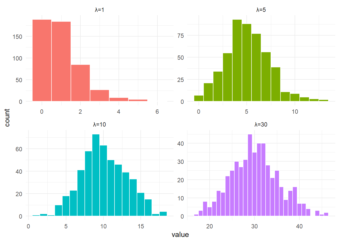
# サンプルを作成。
# なお目的変数作成の係数(a0,b0,lambda0)に意味はなし。
x <- seq(from = 5, to = 35, by = 1)
a0 <- 0.1
b0 <- 0.5
y0 <- exp(b0 + a0 * x)
# 離散カウントデータを目的変数とする。
lambda0 <- 5
y <- round(y0 + rpois(n = length(x), lambda = lambda0))
ggplot() + geom_point(mapping = aes(x = x, y = y), size = 1)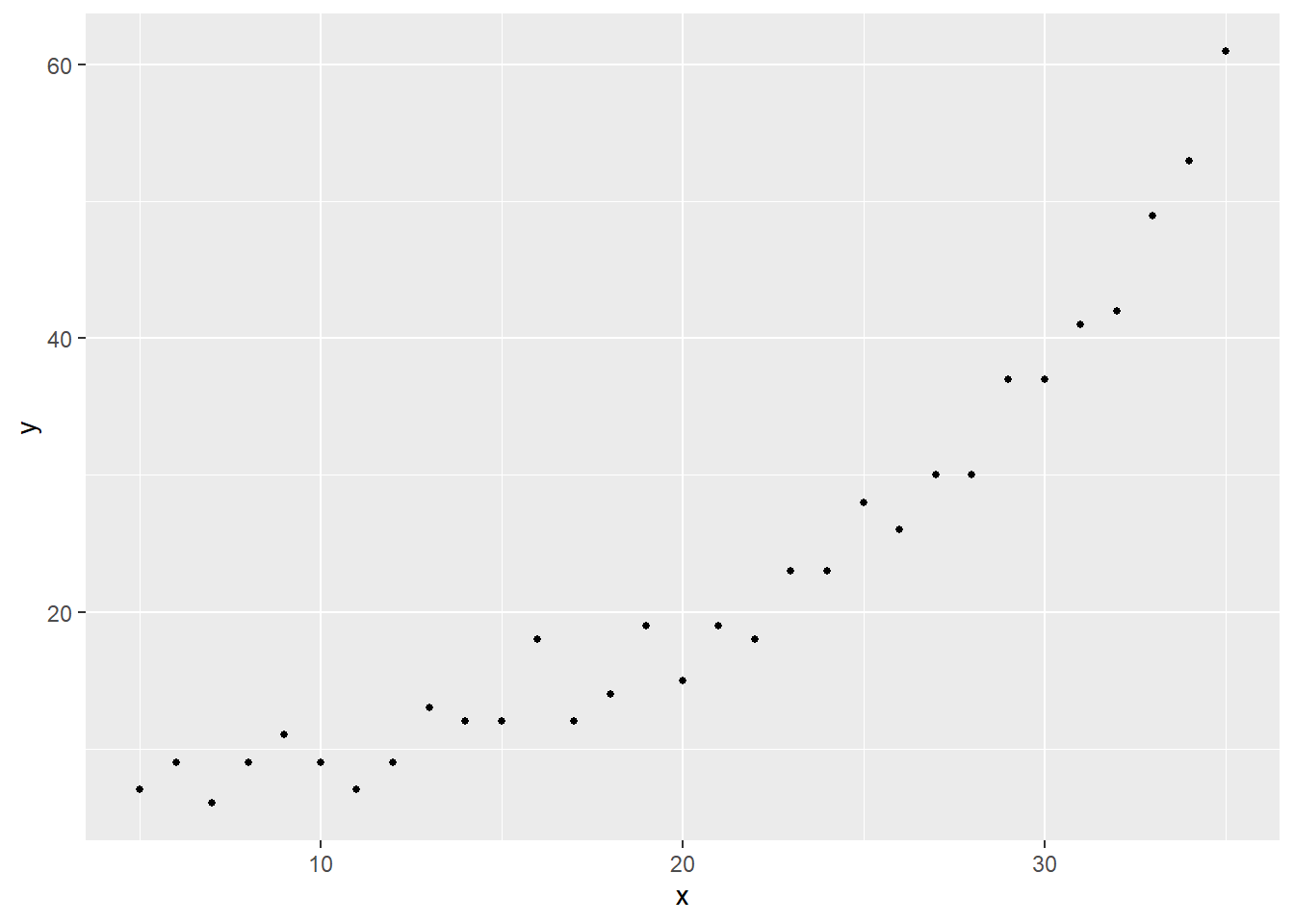
# 誤差構造をポアソン分布、リンク関数を対数関数として一般化線形モデルを解く。
model <- glm(y ~ x, family = poisson(link = "log"))
summary(model)
# 有意な係数
Call:
glm(formula = y ~ x, family = poisson(link = "log"))

Coefficients:
            Estimate Std. Error z value            Pr(>|z|)
(Intercept) 1.449827   0.126796   11.43 <0.0000000000000002 ***
x           0.073044   0.004765   15.33 <0.0000000000000002 ***
---
Signif. codes:  0 '***' 0.001 '**' 0.01 '*' 0.05 '.' 0.1 ' ' 1

(Dispersion parameter for poisson family taken to be 1)

    Null deviance: 273.1666  on 30  degrees of freedom
Residual deviance:   8.5203  on 29  degrees of freedom
AIC: 160.05

Number of Fisher Scoring iterations: 4
# ポアソン回帰のカーブ。
ggplot(mapping = aes(x = x, y = y)) + geom_point(size = 1) + geom_smooth(size = 1, method = "glm", method.args = list(family = poisson(link = "log")), se = T)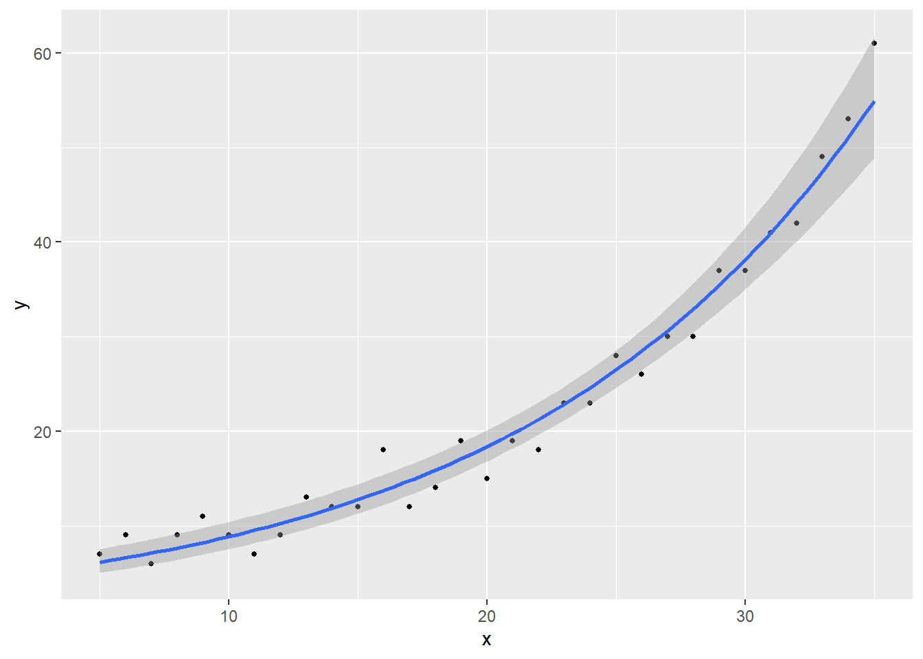
# 推定された係数aの解釈を確認。
# 推定された係数を取り出す。
b <- model$coefficients[1]
a <- model$coefficients[2]
list(a = a, b = b)
$a
x
0.07304358
$b
(Intercept)
1.449827 # その時のy(目的変数)の推定量を確認。
y_hat <- exp(b + a * x)
y_hat [1] 6.141354 6.606730 7.107371 7.645949 8.225340 8.848634 9.519161
[8] 10.240499 11.016497 11.851299 12.749360 13.715473 14.754796 15.872877
[15] 17.075682 18.369633 19.761637 21.259122 22.870084 24.603120 26.467481
[22] 28.473118 30.630737 32.951855 35.448862 38.135085 41.024863 44.133621
[29] 47.477953 51.075710 54.946095# xが1増加すると
result01 <- {
tail(y_hat, -1)/head(y_hat, -1)
} %>%
signif(digits = 6) %>%
unique()yは1.07578倍
# 係数aの指数関数は、
result02 <- exp(a) %>%
    signif(digits = 6)
同じく1.07578となる。
参考引用資料
最終更新
Sys.time()[1] "2024-04-23 08:32:48 JST"R、Quarto、Package
R.Version()$version.string[1] "R version 4.3.3 (2024-02-29 ucrt)"quarto::quarto_version()[1] '1.4.553'packageVersion(pkg = "tidyverse")[1] '2.0.0'