lapply(X = c("dplyr", "pwr", "ggplot2", "scales"), require, character.only = T)Rで確率・統計:サンプルサイズの決定:2変数の相関分析の場合
Rでデータサイエンス
サンプルサイズの決定:2変数の相関分析の場合
2変数の相関の強さの効果量を、ピアソンの積率相関係数とする。
- 相関係数の絶対値が高ければ、決定係数(寄与度、効果)も高い。
相関係数(効果量)、有意水準、サンプルサイズが与えられた場合の検定力算出
- \(\textrm{H}_0:r_c=0\)
# 検定力算出コードは関数から引用
# 効果量(Effect size)
r <- 0.5
# 有意水準
sig.level <- 0.05
# サンプルサイズ
n <- 100
# 標本相関係数 r を絶対値に変換
r <- abs(r)\[t=\dfrac{r\displaystyle\sqrt{n-2}}{\displaystyle\sqrt{1-r^2}}\]が、自由度\(n-2\)の\(t\)分布に従うため、
# 確率が(両側として)有意水準/2、自由度は n-2 に対応する確率点、境界t値を算出
ttt <- qt(sig.level/2, df = n - 2, lower = FALSE)
ttt
[1] 1.984467# 求めた 境界t値 を分位点とする棄却域
g <- ggplot(data = data.frame(x = c(-5, 5)), mapping = aes(x = x)) + theme_minimal() + stat_function(fun = function(x) dt(x = x, df = n - 2), geom = "line", size = 1, n = 200) + geom_vline(xintercept = c(-ttt, ttt)) + scale_x_continuous(breaks = pretty_breaks(10)) + scale_y_continuous(breaks = pretty_breaks(10))
g + stat_function(fun = function(x) dt(x = x, df = n - 2), xlim = c(ttt, 5), geom = "area", fill = "red") + stat_function(fun = function(x) dt(x = x, df = n - 2), xlim = c(-ttt, -5), geom = "area", fill = "red")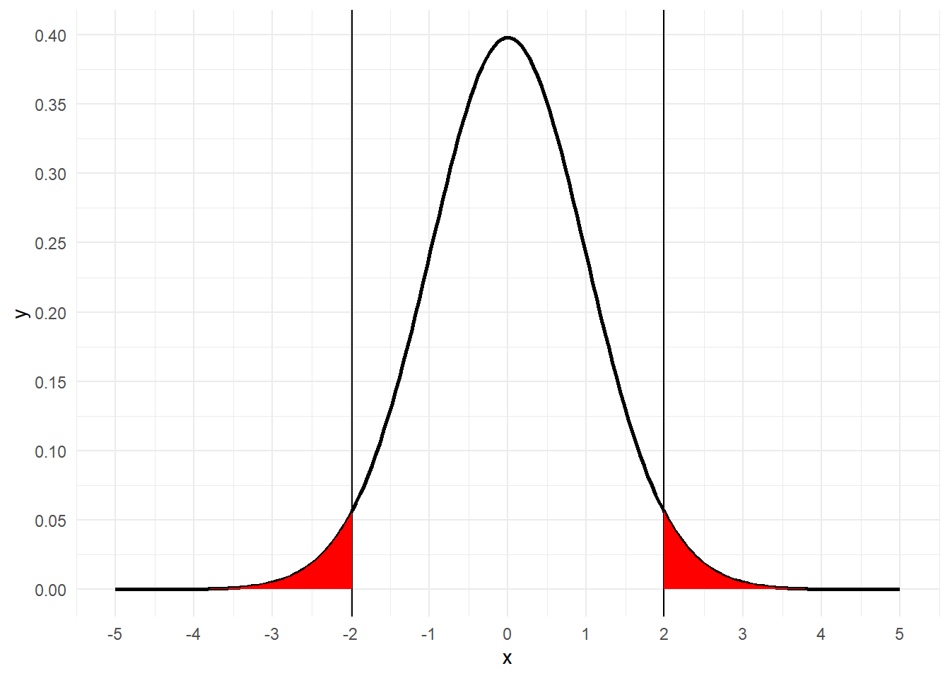
\[t=\dfrac{r\displaystyle\sqrt{n-2}}{\displaystyle\sqrt{1-r^2}},\quad r=\displaystyle\sqrt{\dfrac{t^2}{t^2+n-2}}\]より、
# サンプルサイズと求めた境界t値(ttt)に対応する母相関係数 rc を算出
rc <- sqrt(ttt^2/(ttt^2 + n - 2))
rc
[1] 0.1965512# 標本相関係数 r をフィッシャーのz変換(逆双曲線正接関数)、さらにバイアス補正を加算
zr <- atanh(r) + r/(2 * (n - 1))
zr[1] 0.5518314# 参考としてバイアス補正後のアークタンジェント関数で標本相関係数(0.35、-0.35)を確認
# 垂直線は標本相関係数 r 及び -r
ggplot(data = data.frame(x = c(-0.99, 0.99)), mapping = aes(x = x)) + theme_minimal() + stat_function(fun = function(x) atanh(x) + r/(2 * (n - 1)), geom = "line", size = 1, n = 200) + geom_vline(xintercept = c(-r, r)) + scale_x_continuous(breaks = pretty_breaks(10)) + scale_y_continuous(breaks = pretty_breaks(10))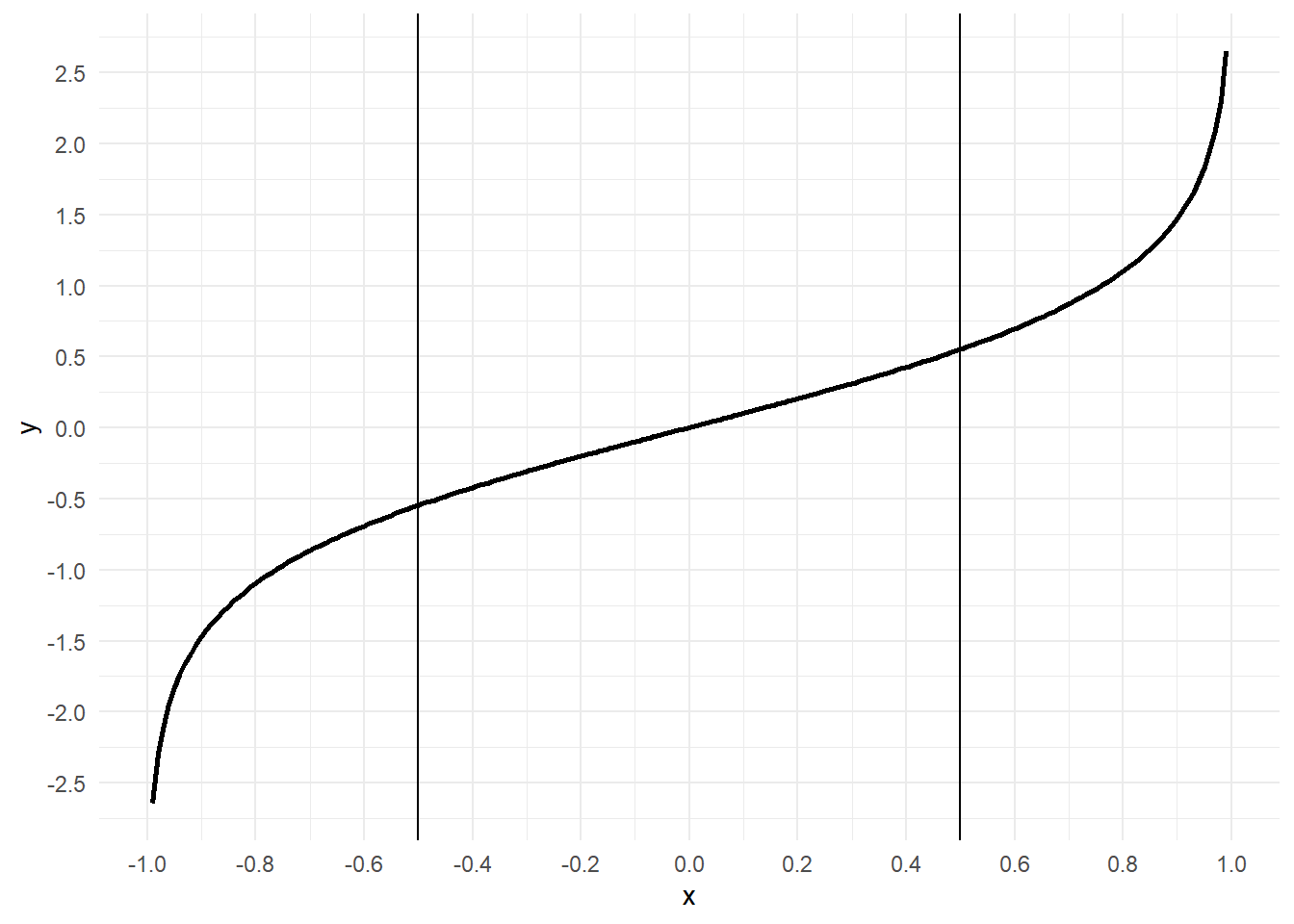
# 母相関係数rcをフィッシャーのz変換
zrc <- atanh(rc)
zrc
[1] 0.1991426「標本相関係数のz変換(zr)が平均を母相関係数のz変換(zrc)、分散を1/(n-3)とする正規分布に近似的に従う」ことから正規化(標準化)したzrを分位点として算出(両側)
# H0としての正規化z値は以下の通り
(zr - zrc) * sqrt(n - 3)
(-zr - zrc) * sqrt(n - 3)
[1] 3.473582
[1] -7.396236# 最後に上記の正規化した zr、-zr を分位点とする確率を求めて合計することによって 1-β 、検定力を求める
# 始めに zr
pnorm((zr - zrc) * sqrt(n - 3))[1] 0.9997432# 確率密度関数
g0 <- ggplot(data = data.frame(x = c(-5, 5)), mapping = aes(x = x)) + theme_minimal() + stat_function(fun = function(x) dnorm(x = x), geom = "line", size = 1, n = 200)
g0 + stat_function(fun = function(x) dnorm(x = x), xlim = c((zr - zrc) * sqrt(n - 3), 0), geom = "area", fill = "red")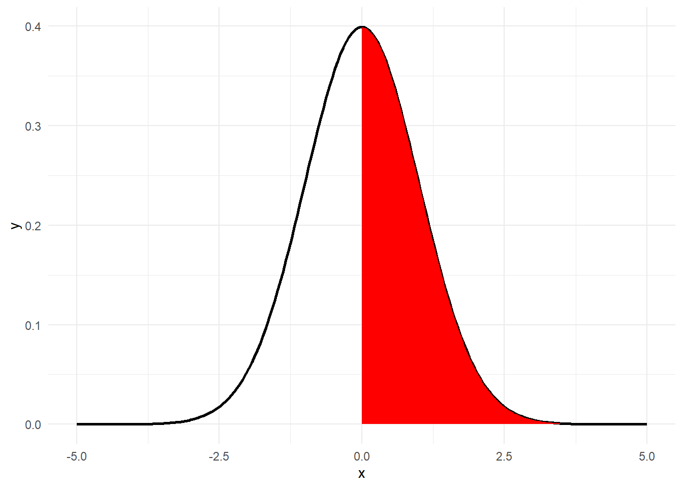
# 次に -zr
pnorm((-zr - zrc) * sqrt(n - 3))
[1] 0.00000000000007004934# 確率密度関数
g0 + stat_function(fun = function(x) dnorm(x = x), xlim = c((-zr - zrc) * sqrt(n - 3), 0), geom = "area", fill = "red")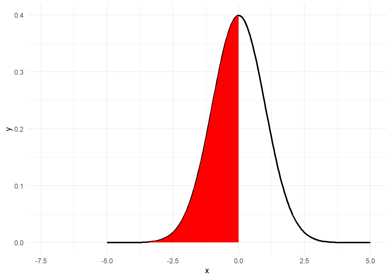
# その合計
power_value <- pnorm((zr - zrc) * sqrt(n - 3)) + pnorm((-zr - zrc) * sqrt(n - 3))
power_value
[1] 0.9997432よって、対立仮説(相関係数がゼロではない)が正しく、かつ帰無仮説(相関係数がゼロ)が棄却される確率は99.974%
# 改めて関数で検定力を確認
result <- pwr.r.test(n = n, r = r, sig.level = 0.05, alternative = "two")
result
{
    result %>%
        plot()
} + geom_hline(yintercept = 0.8) + scale_x_continuous(breaks = pretty_breaks(n = 10)) + scale_y_continuous(breaks = pretty_breaks(n = 10), labels = function(x) paste0(x * 100, "%"))
     approximate correlation power calculation (arctangh transformation)

              n = 100
              r = 0.5
      sig.level = 0.05
          power = 0.9997432
    alternative = two.sided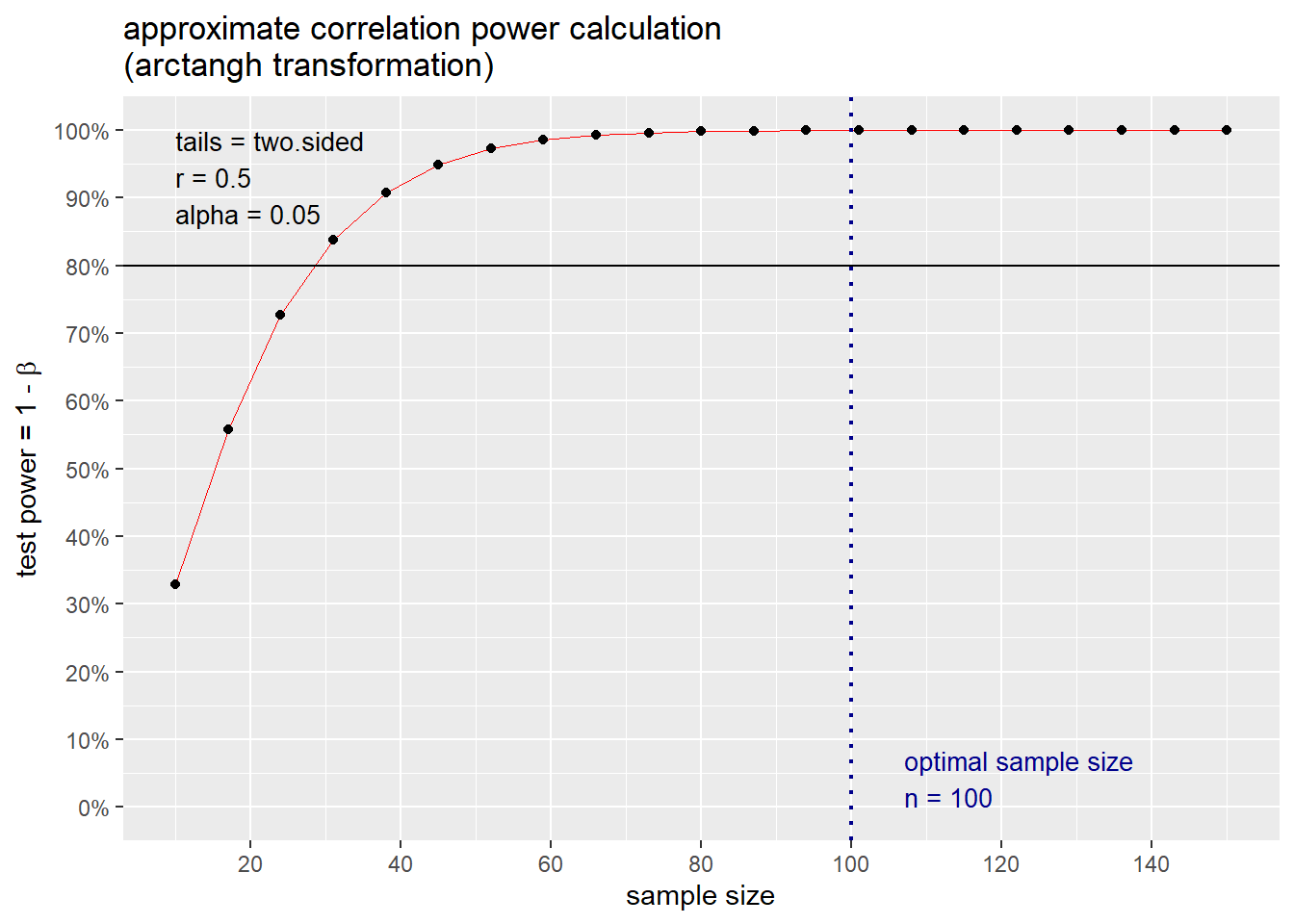
なお、pwr.r.test関数では効果量、有意水準および検定力が与えられた場合、サンプルサイズ n を 4 + 1e-10 から 1e+09の範囲として求めた検定力と与えられた検定力との差がゼロになる n をニュートン法により求めている。
# n <- uniroot(function(n) eval(p.body) - power, c(4 + 1e-10, 1e+09))$rootシミュレーションによるフィッシャーのz変換の確認
library(grid)
func_sim_r <- function(n, a, sd, size, rep) {
    x <- rnorm(n, 0, 1)
    y <- a * x + rnorm(n, 0, sd)
    p <- cor(x, y)
    r <- z <- vector()
    for (i in 1:rep) {
        id <- sample(n, size, replace = F)
        r[i] <- cor(x[id], y[id])
        z[i] <- 1/2 * log((1 + r[i])/(1 - r[i]))
    }
    g1 <- ggplot(mapping = aes(x, y)) + geom_point() + geom_smooth(method = "lm", col = "red") + labs(title = paste0("x と y の散布図. 相関係数 = ", round(p, 3)))
    g2 <- ggplot(mapping = aes(x = r)) + geom_histogram(mapping = aes(y = ..density..), col = "white") + labs(title = paste0("標本相関係数の分布. 平均 = ", round(mean(r), 3)))
    z_df <- data.frame(z = z)
    g3 <- ggplot(data = z_df, mapping = aes(x = z)) + geom_histogram(mapping = aes(y = ..density..), col = "white") + stat_function(fun = dnorm, args = list(mean = 1/2 * log((1 + p)/(1 - p)), sd = 1/sqrt(size - 3)), colour = "red", size = 1) + labs(title = "z変換と近似正規分布")
    gridExtra::grid.arrange(g1, g2, g3, layout_matrix = c(1, 2, 3) %>%
        matrix(nrow = 1)) %>%
        print()
}
n <- 1000
size <- 20
rep <- 2000
a <- 1
sd <- 0.1
func_sim_r(n = n, a = a, sd = sd, size = size, rep = rep)TableGrob (1 x 3) "arrange": 3 grobs
z cells name grob
1 1 (1-1,1-1) arrange gtable[layout]
2 2 (1-1,2-2) arrange gtable[layout]
3 3 (1-1,3-3) arrange gtable[layout]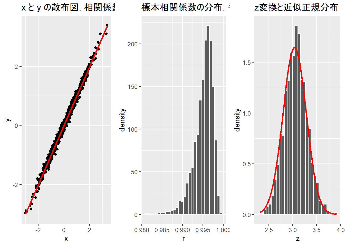
a <- -1
func_sim_r(n = n, a = a, sd = sd, size = size, rep = rep)
TableGrob (1 x 3) "arrange": 3 grobs
z cells name grob
1 1 (1-1,1-1) arrange gtable[layout]
2 2 (1-1,2-2) arrange gtable[layout]
3 3 (1-1,3-3) arrange gtable[layout]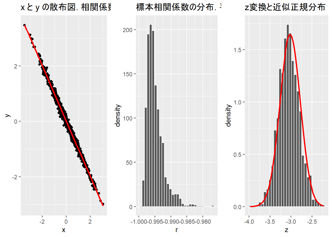
sd <- 2
func_sim_r(n = n, a = a, sd = sd, size = size, rep = rep)
TableGrob (1 x 3) "arrange": 3 grobs
z cells name grob
1 1 (1-1,1-1) arrange gtable[layout]
2 2 (1-1,2-2) arrange gtable[layout]
3 3 (1-1,3-3) arrange gtable[layout]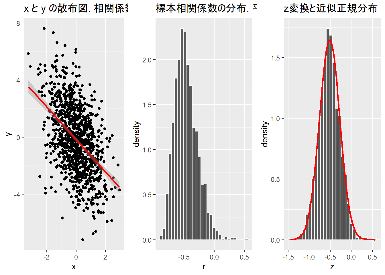
sd <- 4
func_sim_r(n = n, a = a, sd = sd, size = size, rep = rep)
TableGrob (1 x 3) "arrange": 3 grobs
z cells name grob
1 1 (1-1,1-1) arrange gtable[layout]
2 2 (1-1,2-2) arrange gtable[layout]
3 3 (1-1,3-3) arrange gtable[layout]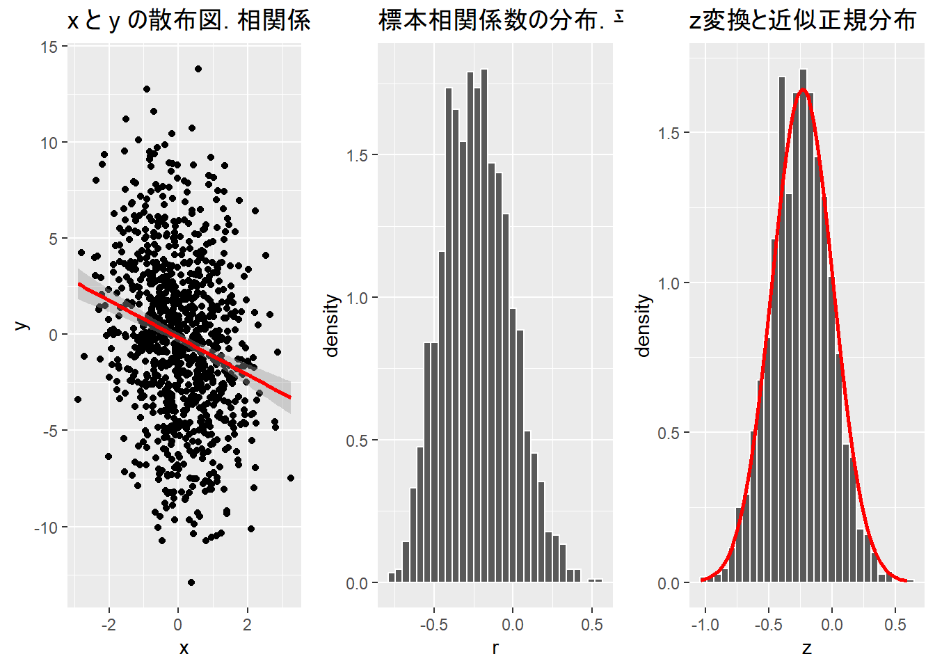
参考引用資料
- Jacob Cohen(1988),『Statistical Power Analysis for the Behavioral Sciences Second Edition』,Lawrence Erlbaum Associates,pp.545-546
- https://cran.r-project.org/web/packages/pwr/pwr.pdf
- https://stackoverflow.com/questions/31215748/how-to-shade-part-of-a-density-curve-in-ggplot-with-no-y-axis-data
- https://www.heisei-u.ac.jp/ba/fukui/pdf/stattext13.pdf
- https://stat.odyssey-com.co.jp/study/pdf/statex/185-190.pdf
- https://www.sas.com/offices/asiapacific/japan/service/technical/faq/list/body/stat086.html
- https://www.sist.ac.jp/~kanakubo/research/statistic/bosoukan.html
- http://hs-www.hyogo-dai.ac.jp/~kawano/HStat/?plugin=cssj&page=2010%2F12th%2FPopulation_Correlation_Coefficien
- https://bellcurve.jp/statistics/course/9591.html
- http://www.igaku-shoin.co.jp/nwsppr/n1997dir/n2241dir/n2241_07.htm
- http://www.cis.kit.ac.jp/~tomaru/pukiwiki/?power_analysis#u188f9b2
最終更新
Sys.time()[1] "2024-04-18 08:51:22 JST"R、Quarto、Package
R.Version()$version.string[1] "R version 4.3.3 (2024-02-29 ucrt)"quarto::quarto_version()[1] '1.4.553'packageVersion(pkg = "tidyverse")[1] '2.0.0'