Analysis
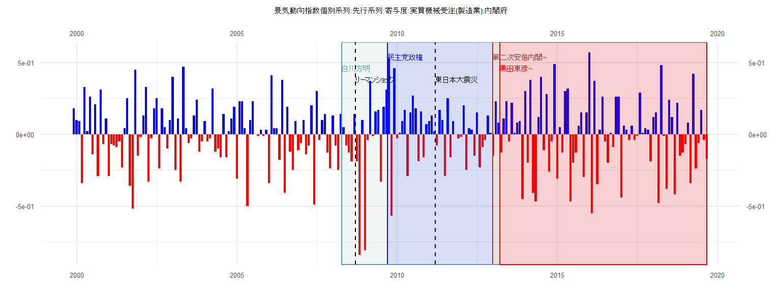
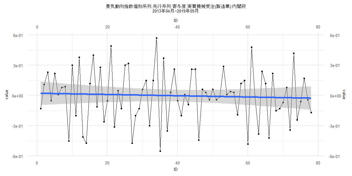
[1] "景気動向指数個別系列:先行系列:寄与度:実質機械受注(製造業):内閣府"
       Jan   Feb   Mar   Apr   May   Jun   Jul   Aug   Sep   Oct   Nov   Dec
1999                                                                    0.18
2000  0.10  0.09 -0.34  0.33  0.02  0.26 -0.14  0.21 -0.29  0.31 -0.07  0.11
2001 -0.29 -0.07 -0.08 -0.09 -0.05 -0.23  0.04  0.25 -0.36 -0.52  0.45 -0.15
2002 -0.02  0.13  0.33 -0.33 -0.03  0.18  0.25 -0.24  0.18  0.05 -0.10  0.10
2003  0.40 -0.25  0.11 -0.33  0.47  0.04 -0.06 -0.03  0.13  0.24 -0.12 -0.05
2004  0.09 -0.05 -0.03  0.32 -0.12 -0.10 -0.16  0.14 -0.16  0.02  0.11  0.19
2005 -0.31  0.23  0.23  0.04 -0.50  0.10  0.23  0.00 -0.01  0.03 -0.01  0.03
2006 -0.34  0.41  0.04  0.04 -0.18  0.38 -0.41  0.19 -0.12 -0.25  0.09 -0.11
2007 -0.06  0.10 -0.14 -0.08  0.20 -0.49  0.30 -0.04  0.10  0.14 -0.13 -0.24
2008  0.13 -0.08 -0.25  0.14  0.05 -0.08 -0.13 -0.19  0.14 -0.19 -0.84  0.10
2009 -0.81 -0.04  0.37 -0.01  0.16  0.17 -0.33  0.19  0.31  0.53 -0.57  0.46
2010 -0.03  0.01  0.09  0.17 -0.29  0.15  0.27  0.18 -0.19  0.16 -0.16  0.07
2011  0.09  0.13  0.02 -0.08  0.17  0.10 -0.29  0.25 -0.16  0.09  0.00 -0.03
2012 -0.02  0.20 -0.25  0.04  0.03 -0.15  0.15 -0.23 -0.09 -0.04  0.13  0.01
2013 -0.15  0.23  0.08 -0.13  0.11  0.23 -0.05  0.22  0.01  0.08  0.09 -0.45
2014  0.30 -0.20  0.38 -0.41 -0.47  0.12  0.40 -0.11  0.28 -0.26 -0.05  0.49
2015 -0.31  0.05 -0.13  0.30  0.32 -0.47 -0.20 -0.13  0.06  0.15 -0.30  0.15
2016  0.57 -0.55  0.37 -0.35  0.03  0.26 -0.05 -0.20  0.01 -0.09  0.26  0.26
2017 -0.44  0.06  0.03 -0.04  0.06 -0.04 -0.01  0.29  0.01  0.04  0.03 -0.19
2018  0.12  0.15 -0.48  0.48 -0.01 -0.38  0.24  0.12 -0.42  0.22 -0.15 -0.13
2019 -0.07  0.08 -0.34  0.42 -0.24 -0.06  0.17 -0.04 -0.17
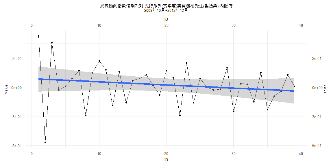
Call:
lm(formula = value ~ ID)

Residuals:
     Min       1Q   Median       3Q      Max
-0.65204 -0.10619  0.03018  0.10894  0.44472

Coefficients:
             Estimate Std. Error t value Pr(>|t|)
(Intercept)  0.088529   0.067208   1.317    0.196
ID          -0.003247   0.002929  -1.109    0.275

Residual standard error: 0.2058 on 37 degrees of freedom
Multiple R-squared:  0.03215,   Adjusted R-squared:  0.005997
F-statistic: 1.229 on 1 and 37 DF,  p-value: 0.2747


    Two-sample Kolmogorov-Smirnov test

data:  lm_residuals and rnorm(n = length(lm_residuals), mean = 0, sd = sd(lm_residuals))
D = 0.10256, p-value = 0.9885
alternative hypothesis: two-sided


    Durbin-Watson test

data:  value ~ ID
DW = 3.0665, p-value = 0.9997
alternative hypothesis: true autocorrelation is greater than 0


    studentized Breusch-Pagan test

data:  value ~ ID
BP = 6.818, df = 1, p-value = 0.009025


    Box-Ljung test

data:  lm_residuals
X-squared = 15, df = 1, p-value = 0.0001075
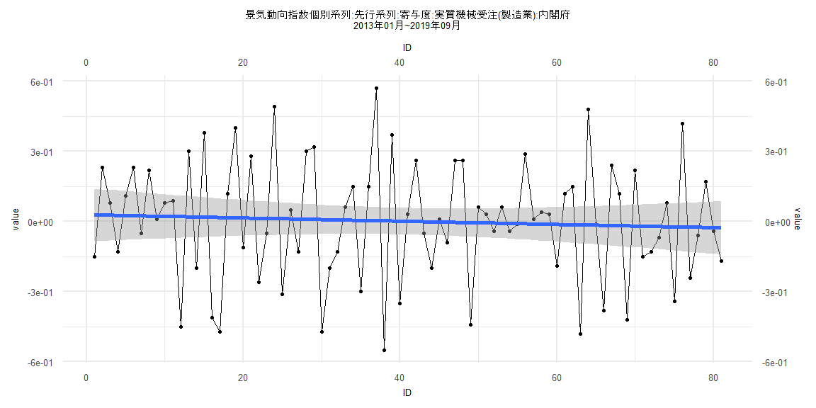
Call:
lm(formula = value ~ ID)

Residuals:
    Min      1Q  Median      3Q     Max
-0.5528 -0.1563  0.0203  0.1955  0.5665

Coefficients:
              Estimate Std. Error t value Pr(>|t|)
(Intercept)  0.0290278  0.0577919   0.502    0.617
ID          -0.0006899  0.0012245  -0.563    0.575

Residual standard error: 0.2577 on 79 degrees of freedom
Multiple R-squared:  0.004003,  Adjusted R-squared:  -0.008605
F-statistic: 0.3175 on 1 and 79 DF,  p-value: 0.5747


    Two-sample Kolmogorov-Smirnov test

data:  lm_residuals and rnorm(n = length(lm_residuals), mean = 0, sd = sd(lm_residuals))
D = 0.14815, p-value = 0.338
alternative hypothesis: two-sided


    Durbin-Watson test

data:  value ~ ID
DW = 2.8258, p-value = 0.9999
alternative hypothesis: true autocorrelation is greater than 0


    studentized Breusch-Pagan test

data:  value ~ ID
BP = 0.27838, df = 1, p-value = 0.5978


    Box-Ljung test

data:  lm_residuals
X-squared = 14.675, df = 1, p-value = 0.0001277
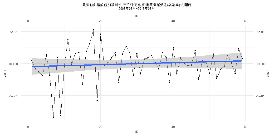
Call:
lm(formula = value ~ ID)

Residuals:
     Min       1Q   Median       3Q      Max
-0.80379 -0.13685  0.01853  0.16047  0.54930

Coefficients:
             Estimate Std. Error t value Pr(>|t|)
(Intercept) -0.046978   0.066334  -0.708    0.482
ID           0.001538   0.001923   0.800    0.427

Residual standard error: 0.2515 on 57 degrees of freedom
Multiple R-squared:  0.01109,   Adjusted R-squared:  -0.006255
F-statistic: 0.6395 on 1 and 57 DF,  p-value: 0.4272


    Two-sample Kolmogorov-Smirnov test

data:  lm_residuals and rnorm(n = length(lm_residuals), mean = 0, sd = sd(lm_residuals))
D = 0.18644, p-value = 0.2582
alternative hypothesis: two-sided


    Durbin-Watson test

data:  value ~ ID
DW = 2.4666, p-value = 0.9545
alternative hypothesis: true autocorrelation is greater than 0


    studentized Breusch-Pagan test

data:  value ~ ID
BP = 5.9013, df = 1, p-value = 0.01513


    Box-Ljung test

data:  lm_residuals
X-squared = 3.4197, df = 1, p-value = 0.06442
Call:
lm(formula = value ~ ID)

Residuals:
     Min       1Q   Median       3Q      Max
-0.55149 -0.15059  0.01653  0.18618  0.56789

Coefficients:
              Estimate Std. Error t value Pr(>|t|)
(Intercept)  0.0230836  0.0596295   0.387    0.700
ID          -0.0006169  0.0013115  -0.470    0.639

Residual standard error: 0.2608 on 76 degrees of freedom
Multiple R-squared:  0.002902,  Adjusted R-squared:  -0.01022
F-statistic: 0.2212 on 1 and 76 DF,  p-value: 0.6395


    Two-sample Kolmogorov-Smirnov test

data:  lm_residuals and rnorm(n = length(lm_residuals), mean = 0, sd = sd(lm_residuals))
D = 0.12821, p-value = 0.546
alternative hypothesis: two-sided


    Durbin-Watson test

data:  value ~ ID
DW = 2.8264, p-value = 0.9999
alternative hypothesis: true autocorrelation is greater than 0


    studentized Breusch-Pagan test

data:  value ~ ID
BP = 0.72088, df = 1, p-value = 0.3959


    Box-Ljung test

data:  lm_residuals
X-squared = 14.126, df = 1, p-value = 0.000171